Model relationships in Power BI Desktop
This article targets import data modelers working with Power BI Desktop. It's an important model design topic that's essential to delivering intuitive, accurate, and optimal models.
For a deeper discussion on optimal model design, including table roles and relationships, see Understand star schema and the importance for Power BI.
Relationship purpose
A model relationship propagates filters applied on the column of one model table to a different model table. Filters will propagate so long as there's a relationship path to follow, which can involve propagation to multiple tables.
Relationship paths are deterministic, meaning that filters are always propagated in the same way and without random variation. Relationships can, however, be disabled, or have filter context modified by model calculations that use particular DAX functions. For more information, see the Relevant DAX functions topic later in this article.
Important
Model relationships don't enforce data integrity. For more information, see the Relationship evaluation topic later in this article, which explains how model relationships behave when there are data integrity issues with your data.
Here's how relationships propagate filters with an animated example.
In this example, the model consists of four tables: Category, Product, Year, and Sales. The Category table relates to the Product table, and the Product table relates to the Sales table. The Year table also relates to the Sales table. All relationships are one-to-many (the details of which are described later in this article).
A query, possibly generated by a Power BI card visual, requests the total sales quantity for sales orders made for a single category, Cat-A, and for a single year, CY2018. It's why you can see filters applied on the Category and Year tables. The filter on the Category table propagates to the Product table to isolate two products that are assigned to the category Cat-A. Then the Product table filters propagate to the Sales table to isolate just two sales rows for these products. These two sales rows represent the sales of products assigned to category Cat-A. Their combined quantity is 14 units. At the same time, the Year table filter propagates to further filter the Sales table, resulting in just the one sales row that is for products assigned to category Cat-A and that was ordered in year CY2018. The quantity value returned by the query is 11 units. Note that when multiple filters are applied to a table (like the Sales table in this example), it's always an AND operation, requiring that all conditions must be true.
Apply star schema design principles
We recommend you apply star schema design principles to produce a model comprising dimension and fact tables. It's common to set up Power BI to enforce rules that filter dimension tables, allowing model relationships to efficiently propagate those filters to fact tables.
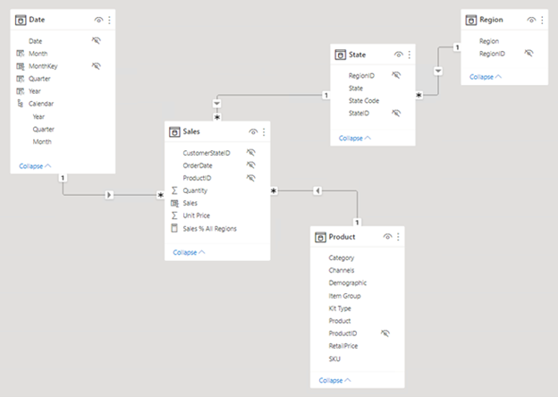
The following image is the model diagram of the Adventure Works sales analysis data model. It shows a star schema design comprising a single fact table named Sales. The other four tables are dimension tables that support the analysis of sales measures by date, state, region, and product. Notice the model relationships connecting all tables. These relationships propagate filters (directly or indirectly) to the Sales table.
Disconnected tables
It's unusual that a model table isn't related to another model table. Such a table in a valid model design is described as a disconnected table. A disconnected table isn't intended to propagate filters to other model tables. Instead, it accepts "user input" (perhaps with a slicer visual), allowing model calculations to use the input value in a meaningful way. For example, consider a disconnected table that's loaded with a range of currency exchange rate values. As long as a filter is applied to filter by a single rate value, a measure expression can use that value to convert sales values.
The Power BI Desktop what-if parameter is a feature that creates a disconnected table. For more information, see Create and use a What if parameter to visualize variables in Power BI Desktop.
Relationship properties
A model relationship relates one column in a table to one column in a different table. (There's one specialized case where this requirement isn't true, and it applies only to multi-column relationships in DirectQuery models. For more information, see the COMBINEVALUES DAX function article.)
Note
It's not possible to relate a column to a different column in the same table. This concept is sometimes confused with the ability to define a relational database foreign key constraint that's table self-referencing. You can use this relational database concept to store parent-child relationships (for example, each employee record is related to a "reports to" employee). However, you can't use model relationships to generate a model hierarchy based on this type of relationship. To create a parent-child hierarchy, see Parent and Child functions.
Data types of columns
The data type for both the "from" and "to' column of the relationship should be the same. Working with relationships defined on DateTime columns might not behave as expected. The engine that stores Power BI data, only uses DateTime data types; Date, Time and Date/Time/Timezone data types are Power BI formatting constructs implemented on top. Any model-dependent objects will still appear as DateTime in the engine (such as relationships, groups, and so on). As such, if a user selects Date from the Modeling tab for such columns, they still don't register as being the same date, because the time portion of the data is still being considered by the engine. Read more about how Date/time types are handled. To correct the behavior, the column data types should be updated in the Power Query Editor to remove the Time portion from the imported data, so when the engine is handling the data, the values will appear the same.
Cardinality
Each model relationship is defined by a cardinality type. There are four cardinality type options, representing the data characteristics of the "from" and "to" related columns. The "one" side means the column contains unique values; the "many" side means the column can contain duplicate values.
Note
If a data refresh operation attempts to load duplicate values into a "one" side column, the entire data refresh will fail.
The four options, together with their shorthand notations, are described in the following bulleted list:
- One-to-many (1:*)
- Many-to-one (*:1)
- One-to-one (1:1)
- Many-to-many (*:*)
When you create a relationship in Power BI Desktop, the designer automatically detects and sets the cardinality type. Power BI Desktop queries the model to know which columns contain unique values. For import models, it uses internal storage statistics; for DirectQuery models it sends profiling queries to the data source. Sometimes, however, Power BI Desktop can get it wrong. It can get it wrong when tables are yet to be loaded with data, or because columns that you expect to contain duplicate values currently contain unique values. In either case, you can update the cardinality type as long as any "one" side columns contain unique values (or the table is yet to be loaded with rows of data).
One-to-many (and many-to-one) cardinality
The one-to-many and many-to-one cardinality options are essentially the same, and they're also the most common cardinality types.
When configuring a one-to-many or many-to-one relationship, you'll choose the one that matches the order in which you related the columns. Consider how you would configure the relationship from the Product table to the Sales table by using the ProductID column found in each table. The cardinality type would be one-to-many, as the ProductID column in the Product table contains unique values. If you related the tables in the reverse direction, Sales to Product, then the cardinality would be many-to-one.
One-to-one cardinality
A one-to-one relationship means both columns contain unique values. This cardinality type isn't common, and it likely represents a suboptimal model design because of the storage of redundant data.
For more information on using this cardinality type, see One-to-one relationship guidance.
Many-to-many cardinality
A many-to-many relationship means both columns can contain duplicate values. This cardinality type is infrequently used. It's typically useful when designing complex model requirements. You can use it to relate many-to-many facts or to relate higher grain facts. For example, when sales target facts are stored at product category level and the product dimension table is stored at product level.
For guidance on using this cardinality type, see Many-to-many relationship guidance.
Note
The Many-to-many cardinality type is supported for models developed for Power BI Report Server January 2024 and later.
Tip
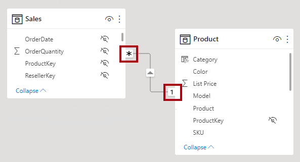
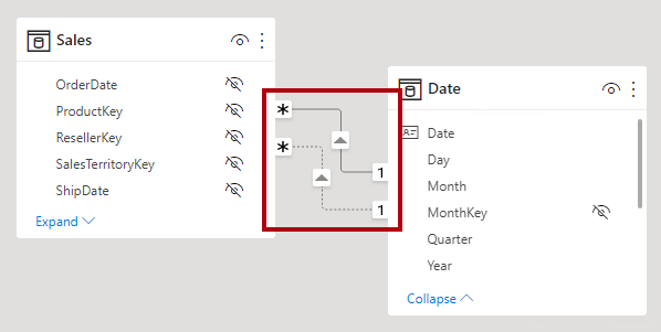
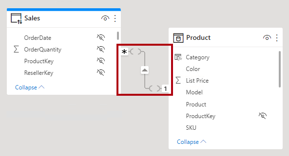
In Power BI Desktop model view, you can interpret a relationship's cardinality type by looking at the indicators (1 or *) on either side of the relationship line. To determine which columns are related, you'll need to select, or hover the cursor over, the relationship line to highlight the columns.
Cross filter direction
Each model relationship is defined with a cross filter direction. Your setting determines the direction(s) that filters will propagate. The possible cross filter options are dependent on the cardinality type.
| Cardinality type | Cross filter options |
|---|---|
| One-to-many (or Many-to-one) | Single Both |
| One-to-one | Both |
| Many-to-many | Single (Table1 to Table2) Single (Table2 to Table1) Both |
Single cross filter direction means "single direction", and Both means "both directions". A relationship that filters in both directions is commonly described as bi-directional.
For one-to-many relationships, the cross filter direction is always from the "one" side, and optionally from the "many" side (bi-directional). For one-to-one relationships, the cross filter direction is always from both tables. Lastly, for many-to-many relationships, cross filter direction can be from either one of the tables, or from both tables. Notice that when the cardinality type includes a "one" side, that filters will always propagate from that side.
When the cross filter direction is set to Both, another property becomes available. It can apply bi-directional filtering when Power BI enforces row-level security (RLS) rules. For more information about RLS, see Row-level security (RLS) with Power BI Desktop.
You can modify the relationship cross filter direction, including the disabling of filter propagation, by using a model calculation. It's achieved by using the CROSSFILTER DAX function.
Bear in mind that bi-directional relationships can impact negatively on performance. Further, attempting to configure a bi-directional relationship could result in ambiguous filter propagation paths. In this case, Power BI Desktop may fail to commit the relationship change and will alert you with an error message. Sometimes, however, Power BI Desktop may allow you to define ambiguous relationship paths between tables. Resolving relationship path ambiguity is described later in this article.
We recommend using bi-directional filtering only as needed. For more information, see Bi-directional relationship guidance.
Tip
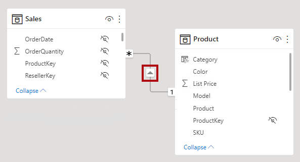
In Power BI Desktop model view, you can interpret a relationship's cross filter direction by noticing the arrowhead(s) along the relationship line. A single arrowhead represents a single-direction filter in the direction of the arrowhead; a double arrowhead represents a bi-directional relationship.
Make this relationship active
There can only be one active filter propagation path between two model tables. However, it's possible to introduce additional relationship paths, though you must set these relationships as inactive. Inactive relationships can only be made active during the evaluation of a model calculation. It's achieved by using the USERELATIONSHIP DAX function.
Generally, we recommend defining active relationships whenever possible. They widen the scope and potential of how report authors can use your model. Using only active relationships means that role-playing dimension tables should be duplicated in your model.
In specific circumstances, however, you can define one or more inactive relationships for a role-playing dimension table. You can consider this design when:
- There's no requirement for report visuals to simultaneously filter by different roles.
- You use the
USERELATIONSHIPDAX function to activate a specific relationship for relevant model calculations.
For more information, see Active vs inactive relationship guidance.
Tip
In Power BI Desktop model view, you can interpret a relationship's active vs inactive status. An active relationship is represented by a solid line; an inactive relationship is represented as a dashed line.
Assume referential integrity
The Assume referential integrity property is available only for one-to-many and one-to-one relationships between two DirectQuery storage mode tables that belong to the same source group. You can only enable this property when the “many” side column doesn't contain NULLs.
When enabled, native queries sent to the data source will join the two tables together by using an INNER JOIN rather than an OUTER JOIN. Generally, enabling this property improves query performance, though it does depend on the specifics of the data source.
Always enable this property when a database foreign key constraint exists between the two tables. Even when a foreign key constraint doesn't exist, consider enabling the property as long as you're certain data integrity exists.
Important
If data integrity should become compromised, the inner join will eliminate unmatched rows between the tables. For example, consider a model Sales table with a ProductID column value that didn't exist in the related Product table. Filter propagation from the Product table to the Sales table will eliminate sales rows for unknown products. This would result in an understatement of the sales results.
For more information, see Assume referential integrity settings in Power BI Desktop.
Relevant DAX functions
There are several DAX functions that are relevant to model relationships. Each function is described briefly in the following bulleted list:
- RELATED: Retrieves the value from "one" side of a relationship. It's useful when involving calculations from different tables that are evaluated in row context.
- RELATEDTABLE: Retrieve a table of rows from "many" side of a relationship.
- USERELATIONSHIP: Allows a calculation to use an inactive relationship. (Technically, this function modifies the weight of a specific inactive model relationship helping to influence its use.) It's useful when your model includes a role-playing dimension table, and you choose to create inactive relationships from this table. You can also use this function to resolve ambiguity in filter paths.
- CROSSFILTER: Modifies the relationship cross filter direction (to one or both), or it disables filter propagation (none). It's useful when you need to change or ignore model relationships during the evaluation of a specific calculation.
- COMBINEVALUES: Joins two or more text strings into one text string. The purpose of this function is to support multi-column relationships in DirectQuery models when tables belong to the same source group.
- TREATAS: Applies the result of a table expression as filters to columns from an unrelated table. It's helpful in advanced scenarios when you want to create a virtual relationship during the evaluation of a specific calculation.
- Parent and Child functions: A family of related functions that you can use to generate calculated columns to naturalize a parent-child hierarchy. You can then use these columns to create a fixed-level hierarchy.
Relationship evaluation
Model relationships, from an evaluation perspective, are classified as either regular or limited. It's not a configurable relationship property. It's in fact inferred from the cardinality type and the data source of the two related tables. It's important to understand the evaluation type because there may be performance implications or consequences should data integrity be compromised. These implications and integrity consequences are described in this topic.
First, some modeling theory is required to fully understand relationship evaluations.
An import or DirectQuery model sources all of its data from either the Vertipaq cache or the source database. In both instances, Power BI is able to determine that a "one" side of a relationship exists.
A composite model, however, can comprise tables using different storage modes (import, DirectQuery or dual), or multiple DirectQuery sources. Each source, including the Vertipaq cache of imported data, is considered to be a source group. Model relationships can then be classified as intra source group or inter/cross source group. An intra source group relationship relates two tables within a source group, while a inter/cross source group relationship relates tables across two source groups. Note that relationships in import or DirectQuery models are always intra source group.
Here's an example of a composite model.
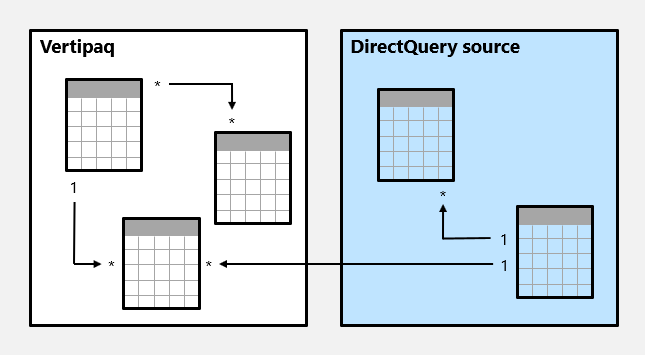
In this example, the composite model consists of two source groups: a Vertipaq source group and a DirectQuery source group. The Vertipaq source group contains three tables, and the DirectQuery source group contains two tables. One cross source group relationship exists to relate a table in the Vertipaq source group to a table in the DirectQuery source group.
Regular relationships
A model relationship is regular when the query engine can determine the "one" side of relationship. It has confirmation that the "one" side column contains unique values. All one-to-many intra source group relationships are regular relationships.
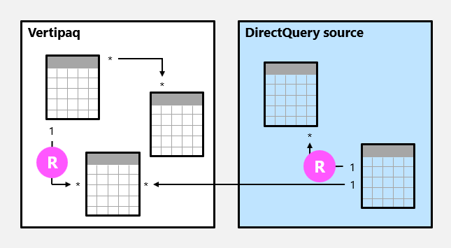
In the following example, there are two regular relationships, both marked as R. Relationships include the one-to-many relationship contained within the Vertipaq source group, and the one-to-many relationship contained within the DirectQuery source.
For import models, where all data is stored in the Vertipaq cache, Power BI creates a data structure for each regular relationship at data refresh time. The data structures consist of indexed mappings of all column-to-column values, and their purpose is to accelerate joining tables at query time.
At query time, regular relationships permit table expansion to happen. Table expansion results in the creation of a virtual table by including the native columns of the base table and then expanding into related tables. For import tables, table expansion is done in the query engine; for DirectQuery tables it's done in the native query that's sent to the source database (as long as the Assume referential integrity property isn't enabled). The query engine then acts upon the expanded table, applying filters and grouping by the values in the expanded table columns.
Note
Inactive relationships are expanded also, even when the relationship isn't used by a calculation. Bi-directional relationships have no impact on table expansion.
For one-to-many relationships, table expansion takes place from the "many" to the "one" sides by using LEFT OUTER JOIN semantics. When a matching value from the "many" to the "one" side doesn't exist, a blank virtual row is added to the "one" side table. This behavior applies only to regular relationships, not to limited relationships.
Table expansion also occurs for one-to-one intra source group relationships, but by using FULL OUTER JOIN semantics. This join type ensures that blank virtual rows are added on either side, when necessary.
Blank virtual rows are effectively unknown members. Unknown members represent referential integrity violations where the "many" side value has no corresponding "one" side value. Ideally these blanks shouldn't exist. They can be eliminated by cleansing or repairing the source data.
Here's how table expansion works with an animated example.

In this example, the model consists of three tables: Category, Product, and Sales. The Category table relates to the Product table with a One-to-many relationship, and the Product table relates to the Sales table with a One-to-many relationship. The Category table contains two rows, the Product table contains three rows, and the Sales tables contains five rows. There are matching values on both sides of all relationships meaning that there are no referential integrity violations. A query-time expanded table is revealed. The table consists of the columns from all three tables. It's effectively a denormalized perspective of the data contained in the three tables. A new row is added to the Sales table, and it has a production identifier value (9) that has no matching value in the Product table. It's a referential integrity violation. In the expanded table, the new row has (Blank) values for the Category and Product table columns.
Limited relationships
A model relationship is limited when there's no guaranteed "one" side. A limited relationship can happen for two reasons:
- The relationship uses a many-to-many cardinality type (even if one or both columns contain unique values).
- The relationship is cross source group (which can only ever be the case for composite models).
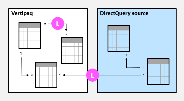
In the following example, there are two limited relationships, both marked as L. The two relationships include the many-to-many relationship contained within the Vertipaq source group, and the one-to-many cross source group relationship.
For import models, data structures are never created for limited relationships. In that case, Power BI resolves table joins at query time.
Table expansion never occurs for limited relationships. Table joins are achieved by using INNER JOIN semantics, and for this reason, blank virtual rows aren't added to compensate for referential integrity violations.
There are other restrictions related to limited relationships:
- The
RELATEDDAX function can't be used to retrieve the "one" side column values. - Enforcing RLS has topology restrictions.
Tip
In Power BI Desktop model view, you can interpret a relationship as being limited. A limited relationship is represented with parenthesis-like marks ( ) after the cardinality indicators.
Resolve relationship path ambiguity
Bi-directional relationships can introduce multiple, and therefore ambiguous, filter propagation paths between model tables. When evaluating ambiguity, Power BI chooses the filter propagation path according to its priority and weight.
Priority
Priority tiers define a sequence of rules that Power BI uses to resolve relationship path ambiguity. The first rule match determines the path Power BI will follow. Each rule below describes how filters flow from a source table to a target table.
- A path consisting of one-to-many relationships.
- A path consisting of one-to-many or many-to-many relationships.
- A path consisting of many-to-one relationships.
- A path consisting of one-to-many relationships from the source table to an intermediate table followed by many-to-one relationships from the intermediate table to the target table.
- A path consisting of one-to-many or many-to-many relationships from the source table to an intermediate table followed by many-to-one or many-to-many relationships from the intermediate table to the target table.
- Any other path.
When a relationship is included in all available paths, it's removed from consideration from all paths.
Weight
Each relationship in a path has a weight. By default, each relationship weight is equal unless the USERELATIONSHIP function is used. The path weight is the maximum of all relationship weights along the path. Power BI uses the path weights to resolve ambiguity between multiple paths in the same priority tier. It won't choose a path with a lower priority but it will choose the path with the higher weight. The number of relationships in the path doesn't affect the weight.
You can influence the weight of a relationship by using the USERELATIONSHIP function. The weight is determined by the nesting level of the call to this function, where the innermost call receives the highest weight.
Consider the following example. The Product Sales measure assigns a higher weight to the relationship between Sales[ProductID] and Product[ProductID], followed by the relationship between Inventory[ProductID] and Product[ProductID].
Product Sales =
CALCULATE(
    CALCULATE(
        SUM(Sales[SalesAmount]),
        USERELATIONSHIP(Sales[ProductID], Product[ProductID])
    ),
    USERELATIONSHIP(Inventory[ProductID], Product[ProductID])
)
Note
If Power BI detects multiple paths that have the same priority and the same weight, it will return an ambiguous path error. In this case, you must resolve the ambiguity by influencing the relationship weights by using the USERELATIONSHIP function, or by removing or modifying model relationships.
Performance preference
The following list orders filter propagation performance, from fastest to slowest performance:
- One-to-many intra source group relationships
- Many-to-many model relationships achieved with an intermediary table and that involve at least one bi-directional relationship
- Many-to-many cardinality relationships
- Cross source group relationships
Related content
For more information about this article, check out the following resources:
- Understand star schema and the importance for Power BI
- One-to-one relationship guidance
- Many-to-many relationship guidance
- Active vs inactive relationship guidance
- Bi-directional relationship guidance
- Relationship troubleshooting guidance
- Video: The Do's and Don'ts of Power BI Relationships
- Questions? Try asking the Power BI Community
- Suggestions? Contribute ideas to improve Power BI
Feedback
Coming soon: Throughout 2024 we will be phasing out GitHub Issues as the feedback mechanism for content and replacing it with a new feedback system. For more information see: https://aka.ms/ContentUserFeedback.
Submit and view feedback for