Excel Conditional Formatting Expiry Dates

Question

Hello,

I'm creating a Excel sheet whereby I have names in a column with skills across the top, I then have the dates that they have completed these skills. I'm trying to set up conditional formatting so that when the date comes within 90 days of today the cell will turn orange and within 30 days the cell will turn red.

For example:

Joe Bloggs has done his eyesight test on the 20/02/2021 which expires after a year, the date today is 06/02/2022 which is within 30 days of expiry, so the cell with the date in will automatically highlight as red.

I've been playing around with the formula below

=AND($B2>TODAY(), $B2-TODAY()<=90)

However this is for if the expiry date has already been calculated. Attached is a screenshot of how I would like it to look

Answer 1

Hi @Ash

Welcome to Q&A forum ~

How do you define “a year”? Can it be represented by 365 days?
If yes, please check whether following conditional formulas are helpful.

Orange : =AND($B2+365-TODAY()>=30,$B2+365-TODAY()<90)
Red : =AND($B2+365-TODAY()>=0,$B2+365-TODAY()<30)

Any misunderstandings, you can let me know.

---

If the answer is helpful, please click "Accept Answer" and kindly upvote it. If you have extra questions about this answer, please click "Comment".
Note: Please follow the steps in our documentation to enable e-mail notifications if you want to receive the related email notification for this thread.

---

Answer 2

Your comment: "Ideally it would work out exactly a year rather than 365 days but that's not too much of an issue, I have noticed however that once it does go past the expiry date the cell will no longer go red and back to the default. An ideas how to rectify that?"

My apologies that I did not interpret your question correctly for my previous post.

However, the following formulas will work and using EDATE for 12 months and will always return exactly a year and takes leap years into account.

Also note that I have applied to the entire column for "Applies to" range so the first cell which is B1 is used in the formula. Remember, as I indicated in my previous post, that the referenced cell is always the first cell of the "Applies to" range.

In the screen shot you will see that dates that have been missed are also red (as per my earlier post)

=AND(NOT(ISBLANK(B1)),EDATE(B1,12)-TODAY()<=30) for the Red format

=AND(NOT(ISBLANK(B1)),EDATE(B1,12)-TODAY()<=90) for the Amber format

Answer 3

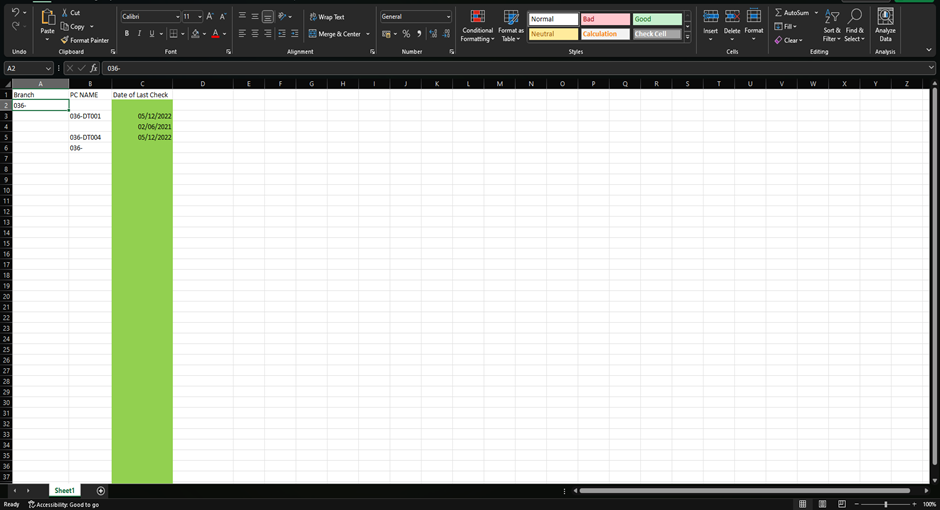
Try the following formulas in the Conditional format.

Note that B3 in the formula is the first cell of the "Applies to" range. By applying the formula to the first cell of the "Applies to" range, Excel looks after applying the formula to the remaining cells in the range.

The NOT(ISBLANK()) is so you can apply the formula to an entire empty column and blank cells will be ignored. However, if you do this, don't forget that B3 in the formula will become B1 as the first cell of the "Applies to" range

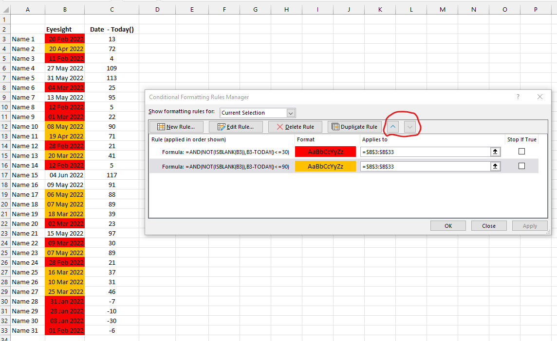
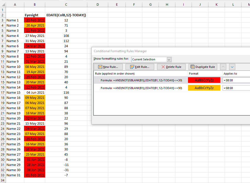
=AND(NOT(ISBLANK(B3)),B3-TODAY()<=30) Use for the red format

=AND(NOT(ISBLANK(B3)),B3-TODAY()<=90) Use for the amber format

As per the screen shot below, ensure that the Red format is the top line in the Rules Manager. Select the line and use Arrow buttons that I have shown with red circle to move the row up or down.

The "Date - Today()" column is for information only so you can check that the correct dates are being formatted. (Today's date Date when creating the formula for this column is 7 Feb 2022). This column plays no part in the conditional format and you do not need it in your project.

Feel free to get back to me if any problems.

Answer 4

Hi, this formula is something I really would love to use but I keep getting this error:

I have not worked with Excel in some time but can't understand why this error occurs.

Any advice?