السابق

التالي

تمرين - تقدير الموارد لمشكلة في العالم الحقيقي

مكتمل

خوارزمية عوامل Shor هي واحدة من الخوارزميات الكمومية الأكثر شهرة. وهو يوفر تسريعا أسيا على أي خوارزمية عوامل كلاسيكية معروفة.

يستخدم التشفير الكلاسيكي وسائل مادية أو رياضية، مثل الصعوبة الحسابية، لإنجاز مهمة. بروتوكول التشفير الشائع هو مخطط Rivest–Shamir-Adleman (RSA)، والذي يستند إلى افتراض صعوبة حساب الأعداد الأولية باستخدام كمبيوتر كلاسيكي.

تشير خوارزمية Shor إلى أن أجهزة الكمبيوتر الكمومية الكبيرة بشكل كاف يمكنها كسر تشفير المفتاح العام. يعد تقدير الموارد المطلوبة لخوارزمية Shor أمرا مهما لتقييم ثغرة هذه الأنواع من مخططات التشفير.

في التمرين التالي، ستحسب تقديرات الموارد لحساب عدد صحيح 2048 بت. بالنسبة لهذا التطبيق، ستقوم بحساب تقديرات الموارد الفعلية مباشرة من تقديرات الموارد المنطقية المحسوبة مسبقا. بالنسبة لميزانية الخطأ المسموح بها، ستستخدم $\epsilon = 1/3$.

كتابة خوارزمية Shor

1. في Visual Studio Code، حدد View > Command palette وحدد Create: New Jupyter Notebook.

2. احفظ دفتر الملاحظات باسم ShorRE.ipynb.

3. في الخلية الأولى، قم باستيراد الحزمة qsharp :

   import qsharp
   

4. Microsoft.Quantum.ResourceEstimation استخدم مساحة الاسم لتعريف إصدار مخزن مؤقتا ومحسن من خوارزمية عوامل العدد الصحيح ل Shor. أضف خلية جديدة وانسخ التعليمات البرمجية التالية والصقها:

   %%qsharp
   open Microsoft.Quantum.Arrays;
   open Microsoft.Quantum.Canon;
   open Microsoft.Quantum.Convert;
   open Microsoft.Quantum.Diagnostics;
   open Microsoft.Quantum.Intrinsic;
   open Microsoft.Quantum.Math;
   open Microsoft.Quantum.Measurement;
   open Microsoft.Quantum.Unstable.Arithmetic;
   open Microsoft.Quantum.ResourceEstimation;
   
   operation RunProgram() : Unit {
       let bitsize = 31;
   
       // When choosing parameters for `EstimateFrequency`, make sure that
       // generator and modules are not co-prime
       let _ = EstimateFrequency(11, 2^bitsize - 1, bitsize);
   }
   
   
   // In this sample we concentrate on costing the `EstimateFrequency`
   // operation, which is the core quantum operation in Shors algorithm, and
   // we omit the classical pre- and post-processing.
   
   /// # Summary
   /// Estimates the frequency of a generator
   /// in the residue ring Z mod `modulus`.
   ///
   /// # Input
   /// ## generator
   /// The unsigned integer multiplicative order (period)
   /// of which is being estimated. Must be co-prime to `modulus`.
   /// ## modulus
   /// The modulus which defines the residue ring Z mod `modulus`
   /// in which the multiplicative order of `generator` is being estimated.
   /// ## bitsize
   /// Number of bits needed to represent the modulus.
   ///
   /// # Output
   /// The numerator k of dyadic fraction k/2^bitsPrecision
   /// approximating s/r.
   operation EstimateFrequency(
       generator : Int,
       modulus : Int,
       bitsize : Int
   )
   : Int {
       mutable frequencyEstimate = 0;
       let bitsPrecision =  2 * bitsize + 1;
   
       // Allocate qubits for the superposition of eigenstates of
       // the oracle that is used in period finding.
       use eigenstateRegister = Qubit[bitsize];
   
       // Initialize eigenstateRegister to 1, which is a superposition of
       // the eigenstates we are estimating the phases of.
       // We first interpret the register as encoding an unsigned integer
       // in little endian encoding.
       ApplyXorInPlace(1, eigenstateRegister);
       let oracle = ApplyOrderFindingOracle(generator, modulus, _, _);
   
       // Use phase estimation with a semiclassical Fourier transform to
       // estimate the frequency.
       use c = Qubit();
       for idx in bitsPrecision - 1..-1..0 {
           within {
               H(c);
           } apply {
               // `BeginEstimateCaching` and `EndEstimateCaching` are the operations
               // exposed by Azure Quantum Resource Estimator. These will instruct
               // resource counting such that the if-block will be executed
               // only once, its resources will be cached, and appended in
               // every other iteration.
               if BeginEstimateCaching("ControlledOracle", SingleVariant()) {
                   Controlled oracle([c], (1 <<< idx, eigenstateRegister));
                   EndEstimateCaching();
               }
               R1Frac(frequencyEstimate, bitsPrecision - 1 - idx, c);
           }
           if MResetZ(c) == One {
               set frequencyEstimate += 1 <<< (bitsPrecision - 1 - idx);
           }
       }
   
       // Return all the qubits used for oracles eigenstate back to 0 state
       // using Microsoft.Quantum.Intrinsic.ResetAll.
       ResetAll(eigenstateRegister);
   
       return frequencyEstimate;
   }
   
   /// # Summary
   /// Interprets `target` as encoding unsigned little-endian integer k
   /// and performs transformation |k⟩ ↦ |gᵖ⋅k mod N ⟩ where
   /// p is `power`, g is `generator` and N is `modulus`.
   ///
   /// # Input
   /// ## generator
   /// The unsigned integer multiplicative order ( period )
   /// of which is being estimated. Must be co-prime to `modulus`.
   /// ## modulus
   /// The modulus which defines the residue ring Z mod `modulus`
   /// in which the multiplicative order of `generator` is being estimated.
   /// ## power
   /// Power of `generator` by which `target` is multiplied.
   /// ## target
   /// Register interpreted as LittleEndian which is multiplied by
   /// given power of the generator. The multiplication is performed modulo
   /// `modulus`.
   internal operation ApplyOrderFindingOracle(
       generator : Int, modulus : Int, power : Int, target : Qubit[]
   )
   : Unit
   is Adj + Ctl {
       // The oracle we use for order finding implements |x⟩ ↦ |x⋅a mod N⟩. We
       // also use `ExpModI` to compute a by which x must be multiplied. Also
       // note that we interpret target as unsigned integer in little-endian
       // encoding by using the `LittleEndian` type.
       ModularMultiplyByConstant(modulus,
                                   ExpModI(generator, power, modulus),
                                   target);
   }
   
   /// # Summary
   /// Performs modular in-place multiplication by a classical constant.
   ///
   /// # Description
   /// Given the classical constants `c` and `modulus`, and an input
   /// quantum register (as LittleEndian) |𝑦⟩, this operation
   /// computes `(c*x) % modulus` into |𝑦⟩.
   ///
   /// # Input
   /// ## modulus
   /// Modulus to use for modular multiplication
   /// ## c
   /// Constant by which to multiply |𝑦⟩
   /// ## y
   /// Quantum register of target
   internal operation ModularMultiplyByConstant(modulus : Int, c : Int, y : Qubit[])
   : Unit is Adj + Ctl {
       use qs = Qubit[Length(y)];
       for (idx, yq) in Enumerated(y) {
           let shiftedC = (c <<< idx) % modulus;
           Controlled ModularAddConstant([yq], (modulus, shiftedC, qs));
       }
       ApplyToEachCA(SWAP, Zipped(y, qs));
       let invC = InverseModI(c, modulus);
       for (idx, yq) in Enumerated(y) {
           let shiftedC = (invC <<< idx) % modulus;
           Controlled ModularAddConstant([yq], (modulus, modulus - shiftedC, qs));
       }
   }
   
   /// # Summary
   /// Performs modular in-place addition of a classical constant into a
   /// quantum register.
   ///
   /// # Description
   /// Given the classical constants `c` and `modulus`, and an input
   /// quantum register (as LittleEndian) |𝑦⟩, this operation
   /// computes `(x+c) % modulus` into |𝑦⟩.
   ///
   /// # Input
   /// ## modulus
   /// Modulus to use for modular addition
   /// ## c
   /// Constant to add to |𝑦⟩
   /// ## y
   /// Quantum register of target
   internal operation ModularAddConstant(modulus : Int, c : Int, y : Qubit[])
   : Unit is Adj + Ctl {
       body (...) {
           Controlled ModularAddConstant([], (modulus, c, y));
       }
       controlled (ctrls, ...) {
           // We apply a custom strategy to control this operation instead of
           // letting the compiler create the controlled variant for us in which
           // the `Controlled` functor would be distributed over each operation
           // in the body.
           //
           // Here we can use some scratch memory to save ensure that at most one
           // control qubit is used for costly operations such as `AddConstant`
           // and `CompareGreaterThenOrEqualConstant`.
           if Length(ctrls) >= 2 {
               use control = Qubit();
               within {
                   Controlled X(ctrls, control);
               } apply {
                   Controlled ModularAddConstant([control], (modulus, c, y));
               }
           } else {
               use carry = Qubit();
               Controlled AddConstant(ctrls, (c, y + [carry]));
               Controlled Adjoint AddConstant(ctrls, (modulus, y + [carry]));
               Controlled AddConstant([carry], (modulus, y));
               Controlled CompareGreaterThanOrEqualConstant(ctrls, (c, y, carry));
           }
       }
   }
   
   /// # Summary
   /// Performs in-place addition of a constant into a quantum register.
   ///
   /// # Description
   /// Given a non-empty quantum register |𝑦⟩ of length 𝑛+1 and a positive
   /// constant 𝑐 < 2ⁿ, computes |𝑦 + c⟩ into |𝑦⟩.
   ///
   /// # Input
   /// ## c
   /// Constant number to add to |𝑦⟩.
   /// ## y
   /// Quantum register of second summand and target; must not be empty.
   internal operation AddConstant(c : Int, y : Qubit[]) : Unit is Adj + Ctl {
       // We are using this version instead of the library version that is based
       // on Fourier angles to show an advantage of sparse simulation in this sample.
   
       let n = Length(y);
       Fact(n > 0, "Bit width must be at least 1");
   
       Fact(c >= 0, "constant must not be negative");
       Fact(c < 2 ^ n, $"constant must be smaller than {2L ^ n}");
   
       if c != 0 {
           // If c has j trailing zeroes than the j least significant bits
           // of y will not be affected by the addition and can therefore be
           // ignored by applying the addition only to the other qubits and
           // shifting c accordingly.
           let j = NTrailingZeroes(c);
           use x = Qubit[n - j];
           within {
               ApplyXorInPlace(c >>> j, x);
           } apply {
               IncByLE(x, y[j...]);
           }
       }
   }
   
   /// # Summary
   /// Performs greater-than-or-equals comparison to a constant.
   ///
   /// # Description
   /// Toggles output qubit `target` if and only if input register `x`
   /// is greater than or equal to `c`.
   ///
   /// # Input
   /// ## c
   /// Constant value for comparison.
   /// ## x
   /// Quantum register to compare against.
   /// ## target
   /// Target qubit for comparison result.
   ///
   /// # Reference
   /// This construction is described in [Lemma 3, arXiv:2201.10200]
   internal operation CompareGreaterThanOrEqualConstant(c : Int, x : Qubit[], target : Qubit)
   : Unit is Adj+Ctl {
       let bitWidth = Length(x);
   
       if c == 0 {
           X(target);
       } elif c >= 2 ^ bitWidth {
           // do nothing
       } elif c == 2 ^ (bitWidth - 1) {
           ApplyLowTCNOT(Tail(x), target);
       } else {
           // normalize constant
           let l = NTrailingZeroes(c);
   
           let cNormalized = c >>> l;
           let xNormalized = x[l...];
           let bitWidthNormalized = Length(xNormalized);
           let gates = Rest(IntAsBoolArray(cNormalized, bitWidthNormalized));
   
           use qs = Qubit[bitWidthNormalized - 1];
           let cs1 = [Head(xNormalized)] + Most(qs);
           let cs2 = Rest(xNormalized);
   
           within {
               for i in IndexRange(gates) {
                   (gates[i] ? ApplyAnd | ApplyOr)(cs1[i], cs2[i], qs[i]);
               }
           } apply {
               ApplyLowTCNOT(Tail(qs), target);
           }
       }
   }
   
   /// # Summary
   /// Internal operation used in the implementation of GreaterThanOrEqualConstant.
   internal operation ApplyOr(control1 : Qubit, control2 : Qubit, target : Qubit) : Unit is Adj {
       within {
           ApplyToEachA(X, [control1, control2]);
       } apply {
           ApplyAnd(control1, control2, target);
           X(target);
       }
   }
   
   internal operation ApplyAnd(control1 : Qubit, control2 : Qubit, target : Qubit)
   : Unit is Adj {
       body (...) {
           CCNOT(control1, control2, target);
       }
       adjoint (...) {
           H(target);
           if (M(target) == One) {
               X(target);
               CZ(control1, control2);
           }
       }
   }
   
   
   /// # Summary
   /// Returns the number of trailing zeroes of a number
   ///
   /// ## Example
   /// ```qsharp
   /// let zeroes = NTrailingZeroes(21); // = NTrailingZeroes(0b1101) = 0
   /// let zeroes = NTrailingZeroes(20); // = NTrailingZeroes(0b1100) = 2
   /// ```
   internal function NTrailingZeroes(number : Int) : Int {
       mutable nZeroes = 0;
       mutable copy = number;
       while (copy % 2 == 0) {
           set nZeroes += 1;
           set copy /= 2;
       }
       return nZeroes;
   }
   
   /// # Summary
   /// An implementation for `CNOT` that when controlled using a single control uses
   /// a helper qubit and uses `ApplyAnd` to reduce the T-count to 4 instead of 7.
   internal operation ApplyLowTCNOT(a : Qubit, b : Qubit) : Unit is Adj+Ctl {
       body (...) {
           CNOT(a, b);
       }
   
       adjoint self;
   
       controlled (ctls, ...) {
           // In this application this operation is used in a way that
           // it is controlled by at most one qubit.
           Fact(Length(ctls) <= 1, "At most one control line allowed");
   
           if IsEmpty(ctls) {
               CNOT(a, b);
           } else {
               use q = Qubit();
               within {
                   ApplyAnd(Head(ctls), a, q);
               } apply {
                   CNOT(q, b);
               }
           }
       }
   
       controlled adjoint self;
   }
   

تقدير خوارزمية Shor

الآن، قم بتقدير الموارد المادية للعملية RunProgram باستخدام الافتراضات الافتراضية. أضف خلية جديدة وانسخ التعليمات البرمجية التالية والصقها:

result = qsharp.estimate("RunProgram()")
result

qsharp.estimate تنشئ الدالة كائن نتيجة يمكنك استخدامه لعرض جدول مع عدد الموارد الفعلية الإجمالية. يمكنك فحص تفاصيل التكلفة عن طريق طي المجموعات التي تحتوي على مزيد من المعلومات.

على سبيل المثال، قم بطي مجموعة معلمات qubit المنطقية لمعرفة أن مسافة التعليمات البرمجية هي 21 وعدد البتات الكمومية الفعلية هو 882.

معلمة qubit المنطقية	القيمة‬
مخطط QEC	surface_code
مسافة التعليمات البرمجية	21
البتات الكمومية الفعلية	882
وقت الدورة المنطقية	8 مللي ثانية
معدل خطأ qubit المنطقي	3.00E-13
عبور Prefactor	0.03
حد تصحيح الخطأ	0.01
صيغة وقت الدورة المنطقية	(4 * twoQubitGateTime + 2 * oneQubitMeasurementTime) * codeDistance
صيغة qubits الفعلية	2 * codeDistance * codeDistance

تلميح

للحصول على إصدار أكثر إحكاما من جدول الإخراج، يمكنك استخدام result.summary.

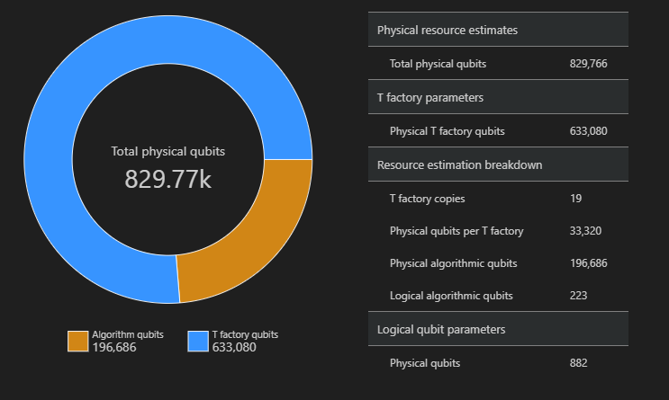
رسم تخطيطي للمساحة

توزيع البتات الكمومية الفعلية المستخدمة للخوارزمية ومصانع T هو عامل قد يؤثر على تصميم الخوارزمية الخاصة بك. يمكنك استخدام الحزمة qsharp-widgets لتصور هذا التوزيع لفهم متطلبات المساحة المقدرة للخوارزمية بشكل أفضل.

from qsharp_widgets import SpaceChart
SpaceChart(result)

في هذا المثال، عدد البتات الكمومية الفعلية المطلوبة لتشغيل الخوارزمية هو 829766، 196686 منها qubits الخوارزمية و633080 منها كيوبتات مصنع T.

مقارنة تقديرات الموارد لتقنيات qubit المختلفة

يسمح لك Azure Quantum Resource Estimator بتشغيل تكوينات متعددة للمعلمات الهدف ومقارنة النتائج. هذا مفيد عندما تريد مقارنة تكلفة نماذج qubit المختلفة أو مخططات QEC أو ميزانيات الخطأ.

يمكنك أيضا إنشاء قائمة بمعلمات التقدير باستخدام EstimatorParams العنصر .

from qsharp.estimator import EstimatorParams, QubitParams, QECScheme, LogicalCounts

labels = ["Gate-based µs, 10⁻³", "Gate-based µs, 10⁻⁴", "Gate-based ns, 10⁻³", "Gate-based ns, 10⁻⁴", "Majorana ns, 10⁻⁴", "Majorana ns, 10⁻⁶"]

params = EstimatorParams(6)
params.error_budget = 0.333
params.items[0].qubit_params.name = QubitParams.GATE_US_E3
params.items[1].qubit_params.name = QubitParams.GATE_US_E4
params.items[2].qubit_params.name = QubitParams.GATE_NS_E3
params.items[3].qubit_params.name = QubitParams.GATE_NS_E4
params.items[4].qubit_params.name = QubitParams.MAJ_NS_E4
params.items[4].qec_scheme.name = QECScheme.FLOQUET_CODE
params.items[5].qubit_params.name = QubitParams.MAJ_NS_E6
params.items[5].qec_scheme.name = QECScheme.FLOQUET_CODE

qsharp.estimate("RunProgram()", params=params).summary_data_frame(labels=labels)

نموذج Qubit	البتات الكمومية المنطقية	العمق المنطقي	حالات T	مسافة التعليمات البرمجية	مصانع T	كسر مصنع T	البتات الكمومية الفعلية	rQOPS	وقت التشغيل الفعلي
μs المستندة إلى البوابة، 10⁻³	223 3.64 مليون	4.70 مليون	17	13	40.54 %	216.77 ألف	21.86 ألف	10 ساعات
μs المستندة إلى البوابة، 10⁻⁴	223	3.64 مليون	4.70 مليون	9	14	43.17 %	63.57 ألف	41.30 ألف	خمس ساعات
ns المستندة إلى البوابة، 10⁻³	223 3.64 مليون	4.70 مليون	17	16	69.08 %	416.89 ألف	32.79 مليون	25 ثانية
ns المستندة إلى البوابة، 10⁻⁴	223 3.64 مليون	4.70 مليون	9	14	43.17 %	63.57 ألف	61.94 مليون	13 ثانية
Majorana ns, 10⁻⁴	223 3.64 مليون	4.70 مليون	9	19	82.75 %	501.48 ألف	82.59 مليون	10 ثوان
Majorana ns, 10⁻⁶	223 3.64 مليون	4.70 مليون	5	13	31.47 %	42.96 ألف	148.67 مليون	5 ثوان

استخراج تقديرات الموارد من عدد الموارد المنطقية

إذا كنت تعرف بالفعل بعض التقديرات لعملية ما، يسمح لك "مقدر الموارد" بدمج التقديرات المعروفة في تكلفة البرنامج الإجمالية لتقليل وقت التنفيذ. يمكنك استخدام LogicalCounts الفئة لاستخراج تقديرات الموارد المنطقية من قيم تقدير الموارد المحسوبة مسبقا.

حدد Code لإضافة خلية جديدة، ثم أدخل التعليمات البرمجية التالية وقم بتشغيلها:

logical_counts = LogicalCounts({
    'numQubits': 12581,
    'tCount': 12,
    'rotationCount': 12,
    'rotationDepth': 12,
    'cczCount': 3731607428,
    'measurementCount': 1078154040})

logical_counts.estimate(params).summary_data_frame(labels=labels)

نموذج Qubit	البتات الكمومية المنطقية	العمق المنطقي	حالات T	مسافة التعليمات البرمجية	مصانع T	كسر مصنع T	البتات الكمومية الفعلية	وقت التشغيل الفعلي
μs المستندة إلى البوابة، 10⁻³	25481	1.2e+10	1.5e+10	27	13	0.6%	37.38 مليون	6 سنوات
μs المستندة إلى البوابة، 10⁻⁴	25481	1.2e+10	1.5e+10	13	14	0.8%	8.68 مليون	3 أعوام
ns المستندة إلى البوابة، 10⁻³	25481	1.2e+10	1.5e+10	27	15	1.3%	37.65 مليون	يومان
ns المستندة إلى البوابة، 10⁻⁴	25481	1.2e+10	1.5e+10	13	18	1.2%	8.72 مليون	18 ساعة
Majorana ns, 10⁻⁴	25481	1.2e+10	1.5e+10	15	15	1.3%	26.11 مليون	15 ساعات
Majorana ns, 10⁻⁶	25481	1.2e+10	1.5e+10	7	13	0.5%	6.25 مليون	7 ساعات

الخاتمة

في أسوأ السيناريوهات، سيحتاج الكمبيوتر الكمومي الذي يستخدم كيوبتات μs المستندة إلى البوابة (qubits التي لها أوقات تشغيل في نظام nanosecond، مثل qubits فائقة التوصيل) ورمز QEC surface إلى ست سنوات و37.38 مليون كيوبتات لعامل عدد صحيح 2048 بت باستخدام خوارزمية Shor.

إذا كنت تستخدم تقنية qubit مختلفة - على سبيل المثال، qubits ns ion المستندة إلى البوابة - ونفس رمز السطح، فإن عدد البتات الكمومية لا يتغير كثيرا، ولكن يصبح وقت التشغيل يومين في أسوأ الحالات و18 ساعة في الحالة المتفائلة. إذا قمت بتغيير تقنية qubit ورمز QEC - على سبيل المثال، باستخدام qubits المستندة إلى Majorana - يمكن إجراء حساب عدد صحيح 2048 بت باستخدام خوارزمية Shor في ساعات مع صفيف من 6.25 ملايين كيوبت في سيناريو أفضل حالة.

من تجربتك، يمكنك استنتاج أن استخدام Qubits Majorana ورمز Floquet QEC هو الخيار الأفضل لتنفيذ خوارزمية Shor وعامل عدد صحيح 2048 بت.

متابعة