Design forecast models

Forecast models let you arrange and configure tiles to define the forecast that's made by a forecast profile. Each model presents a flowchart that graphically represents the calculation that the model does.

Demand forecasting algorithms

Demand planning includes three popular demand forecasting algorithms: auto-ARIMA, ETS, and Prophet. The demand forecasting algorithm that you use depends on the specific characteristics of your historical data.

• Auto-ARIMA works best when data follows stable patterns.
• Error, trend, and seasonality (ETS) is a versatile choice for data that has trends or seasonality.
• Prophet works best with complex, real-world data.

Demand planning also provides both a best fit model (which automatically selects the best of the available algorithms for each product and dimension combination) and the ability to develop and use your own custom models.

By understanding these algorithms and their strengths, you can make informed decisions to optimize your supply chain and meet customer demand.

This section describes how each algorithm works and its suitability for different types of historical demand data.

Best fit model

The best fit model automatically finds which of the other available algorithms (auto-ARIMA, ETS, or Prophet) best fits your data for each product and dimension combination. In this way, different models can be used for different products. In most cases, we recommend using the best fit model because it combines the strengths of all of the other standard models. The following example shows how.

Suppose you have the historical demand time-series data that includes the dimension combinations listed in the following table.

Product	Store
A	1
A	2
B	1
B	2

When you run a forecast calculation using the Prophet model, you get the following results. In this example, the system always uses the Prophet model, regardless of the calculated mean absolute percentage error (MAPE) for each product and dimension combination.

Product	Store	forecast model	MAPE
A	1	Prophet	0.12
A	2	Prophet	0.56
B	1	Prophet	0.65
B	2	Prophet	0.09

When you run a forecast calculation using the ETS model, you get the following results. In this example, the system always uses the ETS model, regardless of the calculated MAPE for each product and dimension combination.

Product	Store	forecast model	MAPE
A	1	ETS	0.18
A	2	ETS	0.15
B	1	ETS	0.21
B	2	ETS	0.31

When you run a forecast calculation using the best fit model, the system optimizes the model selection for each product and dimension combination. The selection changes based on patterns found in the historical sales data.

Product	Store	Prophet MAPE	Auto-ARIMA MAPE	ETS MAPE	Best fit forecast model	Best fit MAPE
A	1	0.12	0.34	0.18	Prophet	0.12
A	2	0.56	0.23	0.15	ETS	0.15
B	1	0.65	0.09	0.21	Auto-ARIMA	0.09
B	2	0.10	0.27	0.31	Prophet	0.10

The following graph shows the overall sales forecast across all dimensions (all products in all stores) over the next nine months, found using three different forecast models. The green line represents the best fit model. Because best fit chooses the best forecast model for each product and dimension combination, it avoids the outliers that could occur from forcing a single model on all dimension combinations. As a result, the overall best-fit forecast resembles an average of the single-model forecasts.

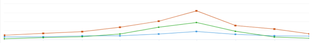
Legend:

• Red = Only Prophet
• Blue = Only ETS
• Green = Best fit

Auto-ARIMA: The time traveler's delight

The auto-ARIMA algorithm is like a time machine: it takes you on a journey through past demand patterns so that you can make informed predictions about the future. Auto-ARIMA uses a technique that's known as autoregressive integrated moving average (ARIMA). This technique combines three key components: autoregression, differencing, and moving averages. The auto-ARIMA algorithm automatically identifies the best combination of these components to create a forecast model that suits your data.

Auto-ARIMA works especially well with time series data that shows a stable pattern over time, such as seasonal fluctuations or trends. If your historical demand follows a reasonably consistent path, auto-ARIMA might be your preferred forecasting method.

ETS: The shape shifter

Error, trend, and seasonality (ETS) is a versatile demand forecasting algorithm that adapts to the shape of your data. It can change its approach based on the characteristics of your historical demand. Therefore, it's suitable for a wide range of scenarios.

The name ETS is an abbreviation for the three essential components that the algorithm decomposes the time series data into: error, trend, and seasonality. By understanding and modeling these components, ETS generates forecasts that capture the underlying patterns in your data. It works best with data that shows clear seasonal patterns, trends, or both. Therefore, it's an excellent choice for businesses that have seasonally affected products or services.

Prophet: The visionary forecasting guru

Prophet was developed by Facebook's research team. It's a modern and flexible forecasting algorithm that can handle the challenges of real-world data. It's especially effective at handling missing values, outliers, and complex patterns.

Prophet works by decomposing the time series data into several components, such as trend, seasonality, and holidays, and then fitting a model to each component. This approach enables Prophet to accurately capture the nuances in your data and produce reliable forecasts. Prophet is ideal for businesses that have irregular demand patterns or frequent outliers, or businesses that are affected by special events such as holidays or promotions.

Custom Azure Machine Learning algorithm

If you have a custom Microsoft Azure Machine Learning algorithm that you want to use with your forecasting models, you can use it in Demand planning.

Create and customize a forecast model

To create and customize a forecast model, you must first open an existing forecast profile. (For more information, see Work with forecast profiles.) You can then fully customize the model that the selected profile uses by adding, removing, and arranging tiles, and configuring settings for each of them.

Follow these steps to create and customize a forecast model.

1. On the navigation pane, select Operations > Forecast profiles.
2. Select the forecast profile that you want to create or customize a forecast model for.
3. On the Forecast model tab, there will always be at least one tile (of the Input type) at the top of the flow chart. The model is processed from top to bottom, and the last tile must be a tile of the Save type. Add, remove, and arrange tiles as you require, and configure settings for each of them. For guidelines, see the illustration after this procedure.
4. When you've finished designing your forecast model, select the Validate button in the upper-right corner. The system runs a few tests to validate that your model will work, and then provides feedback. Fix any issues that the validation test reports.
5. Continue to work until your model is ready. Then, on the Action Pane, select Save.
6. If you want to save your forecast model as a preset, so that it's available when you and other users create a new forecast profile, select the Save as model template button in the upper-right corner.

The following illustration shows the information and controls that are available for tiles in a forecast model.

Legend:

1. Tile icon – A symbol that represents the purpose of the tile.

2. Tile type – The type of tile. This text usually describes the type of roles, calculations, or other actions that the tile represents.

3. Tile name – The name that's applied to the tile. Sometimes, you can enter manually this text in the tile's settings. However, it usually indicates the value of one of the settings that were configured for the tile.

4. Tile actions – Open a menu of actions that you can take on the tile. Although some of these actions are specific to the tile type, most are common to all tiles. If any actions appear dimmed, they can't be used because of the tile's current position or for some other contextual reason. Here are some common actions that are available:

   • Settings – Open a dialog box where you can configure settings for the tile.
   • Remove – Remove the tile.
   • Move Up and Move Down – Reposition the tile in the flowchart.
   • Set to 'Pass Through' – Temporarily disable a currently enabled tile without deleting it or its settings.
   • Unset 'Pass Through' – Reenable a currently disabled tile.

5. Add a tile – Add a new tile at the selected location.

Forecast tile types

This section describes the purpose of each type of forecast tile. It also explains how to use and configure each type.

Input tiles

Input tiles represent the time series that provides input to the forecast model. The time series is the one that's listed on the Included tab of the Input Data tab. You can't edit the name.

Input tiles have just one field that you can set: Fill missing values.

Handle outliers tiles

Handle outliers tiles identify and compensate for outlier data points in the input. These data points are considered anomalies that should be ignored or smoothed out to prevent them from throwing off the forecast calculation.

Handle outliers tiles have the following fields that you can set:

• Handle outliers – Select one of the following options:

  • Interquartile range (IQR)
  • Seasonal and trend decomposition using loess (STL)

• Interquartile range multiplier – This field is available only when the Handle outliers field is set to IQR.

• Correction methods – This field is available only when the Handle outliers field is set to IQR.

• Seasonality hint – This field is available only when the Handle outliers field is set to STL.

Forecast tiles

Forecast tiles apply a selected forecast algorithm to the input time series to create a forecast time series.

Forecast tiles have just one field that you can set: Model type. Use it to select the forecast algorithm to use. For more information about each of the available algorithms, see the Demand forecasting algorithms section. Select one of the following algorithms:

• ARIMA – Autoregressive integrated moving average
• ETS – Error, trend, seasonality
• Prophet – Facebook Prophet
• Best fit model

Finance and operations – Azure Machine Learning tiles

If you're already using your own Azure Machine Learning algorithms for demand forecasting in Supply Chain Management (as described in Demand forecasting overview), you can continue to use them while you use Demand planning. Just put a Finance and operations – Azure Machine Learning tile in your forecast model instead of a Forecast tile.

For information about how to set up Demand planning to connect to and use your Azure Machine Learning algorithms, see Use your own custom Azure Machine Learning algorithms in Demand planning.

Phase in/out tiles

Phase in/out tiles modify the values of a data column in a time series to simulate the gradual phasing in of a new element (such as a new product or warehouse) or phasing out of an old element. The phase in/out calculation lasts for a specific period and uses values that are drawn from the same time series (from either the same data column that is being adjusted or another data column that represents a similar element).

Phase in/out tiles have the following fields that you can set:

• Step name – The specific name of the tile. This name is also shown in the flowchart.
• Description – A short description of the tile.
• Created by – The user who created the tile.
• Rule group – The name of the rule group that defines the calculation that the tile does.

When you set up your forecast model, the position of the Phase in/out tile affects the calculation result. To apply the phase in/out calculation to the historical sales numbers, put the Phase in/out tile before the Forecast tile (as shown on the left side of the following illustration). To apply the phase in/out calculation to the forecasted result, put the Phase in/out tile after the Forecast tile (as shown on the right side of the following illustration).

For more information about phase in/out functionality, including details about how to set up your phase in/out rule groups, see Use phase in/out functionality to simulate planned changes.

Save tiles

Save tiles save the result of the forecast model as a new or updated series. All forecast models must end with a single Save tile.

The forecast time series will be saved according to the settings that you configure each time that you run a forecast job as described in Work with forecast profiles.