TartanAir: AirSim simulation dataset for simultaneous localization and mapping (SLAM)
Simultaneous Localization and Mapping (SLAM) is one of the most fundamental capabilities necessary for robots. Due to the ubiquitous availability of images, Visual SLAM (V-SLAM) has become an important component of many autonomous systems. Impressive progress has been made with both geometric-based methods and learning-based methods. However, developing robust and reliable SLAM methods for real-world applications is still a challenging problem. Real-life environments are full of difficult cases such as light changes or lack of illumination, dynamic objects, and texture-less scenes. This dataset takes advantages of the advancing computer graphics technology, and aims to cover diverse scenarios with challenging features in simulation.
Note
Microsoft provides Azure Open Datasets on an “as is” basis. Microsoft makes no warranties, express or implied, guarantees or conditions with respect to your use of the datasets. To the extent permitted under your local law, Microsoft disclaims all liability for any damages or losses, including direct, consequential, special, indirect, incidental or punitive, resulting from your use of the datasets.
This dataset is provided under the original terms that Microsoft received source data. The dataset may include data sourced from Microsoft.
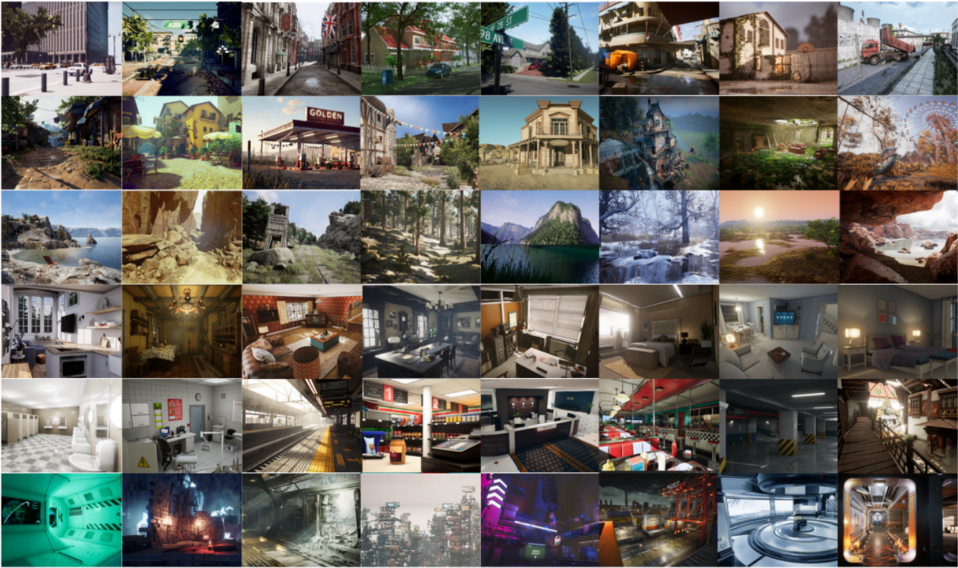
The data is collected in photo-realistic simulation environments in the presence of various light conditions, weather, and moving objects. By collecting data in simulation, we are able to obtain multi-modal sensor data and precise ground truth labels, including the stereo RGB image, depth image, segmentation, optical flow, and camera poses. We set up a large number of environments with various styles and scenes, covering challenging viewpoints and diverse motion patterns, which are difficult to achieve by using physical data collection platforms. The four most important features of our dataset are: 1) Large-size diverse realistic data; 2) Multimodal ground truth labels; 3) Diversity of motion patterns; 4) Challenging Scenes.
This dataset provides five types of data:
- Stereo images: image type (PNG)
- Depth file: numpy type (NPY)
- Segmentation file: numpy type (NPY)
- Optical flow file: numpy type (NPY)
- Camera pose file: text type (TXT)
It is collected from different environments, contains hundreds of trajectories (3 TB) in total as of 2019.
Challenging visual effects
In some simulations, The dataset simulates multiple types of challenging visual effects.
- Hard lighting conditions. Day-night alternating. Low-lighting. Rapidly changing illuminations.
- Weather effects. Clear, raining, snowing, windy, and fog.
- Seasonal change.
Storage location
This dataset is stored in the East US Azure region. Allocating compute resources in East US is recommended for affinity.
License terms
This project is released under the MIT License. Review the License file for more details.
Additional information
View the official TartanAir website or view the original research paper.
Email tartanair@hotmail.com if you have any questions about the data source. You can also reach out to contributers on the associated GitHub.
Citation More technical details are available in AirSim paper (FSR 2017 Conference). Cite this as:
@article{tartanair2020arxiv,
  title =   {TartanAir: A Dataset to Push the Limits of Visual SLAM},
  author =  {Wenshan Wang, Delong Zhu, Xiangwei Wang, Yaoyu Hu, Yuheng Qiu, Chen Wang, Yafei Hu, Ashish Kapoor, Sebastian Scherer},
  journal = {arXiv preprint arXiv:2003.14338},
  year =    {2020},
  url = {https://arxiv.org/abs/2003.14338}
}
@inproceedings{airsim2017fsr,
  author = {Shital Shah and Debadeepta Dey and Chris Lovett and Ashish Kapoor},
  title = {AirSim: High-Fidelity Visual and Physical Simulation for Autonomous Vehicles},
  year = {2017},
  booktitle = {Field and Service Robotics},
  eprint = {arXiv:1705.05065},
  url = {https://arxiv.org/abs/1705.05065}
}
Data access
Use the following code sample to access the data in a Python notebook.
Dependencies
pip install numpy
pip install azure-storage-blob
pip install opencv-python
Imports and container client
from azure.storage.blob import ContainerClient
import numpy as np
import io
import cv2
import time
import matplotlib.pyplot as plt
%matplotlib inline

# Dataset website: http://theairlab.org/tartanair-dataset/
account_url = 'https://tartanair.blob.core.windows.net/'
container_name = 'tartanair-release1'

container_client = ContainerClient(account_url=account_url,
                                 container_name=container_name,
                                 credential=None)
Environments and trajectories
def get_environment_list():
    '''
    List all the environments shown in the root directory
    '''
    env_gen = container_client.walk_blobs()
    envlist = []
    for env in env_gen:
        envlist.append(env.name)
    return envlist

def get_trajectory_list(envname, easy_hard = 'Easy'):
    '''
    List all the trajectory folders, which is named as 'P0XX'
    '''
    assert(easy_hard=='Easy' or easy_hard=='Hard')
    traj_gen = container_client.walk_blobs(name_starts_with=envname + '/' + easy_hard+'/')
    trajlist = []
    for traj in traj_gen:
        trajname = traj.name
        trajname_split = trajname.split('/')
        trajname_split = [tt for tt in trajname_split if len(tt)>0]
        if trajname_split[-1][0] == 'P':
            trajlist.append(trajname)
    return trajlist

def _list_blobs_in_folder(folder_name):
    """
    List all blobs in a virtual folder in an Azure blob container
    """

    files = []
    generator = container_client.list_blobs(name_starts_with=folder_name)
    for blob in generator:
        files.append(blob.name)
    return files

def get_image_list(trajdir, left_right = 'left'):
    assert(left_right == 'left' or left_right == 'right')
    files = _list_blobs_in_folder(trajdir + '/image_' + left_right + '/')
    files = [fn for fn in files if fn.endswith('.png')]
    return files

def get_depth_list(trajdir, left_right = 'left'):
    assert(left_right == 'left' or left_right == 'right')
    files = _list_blobs_in_folder(trajdir + '/depth_' + left_right + '/')
    files = [fn for fn in files if fn.endswith('.npy')]
    return files

def get_flow_list(trajdir, ):
    files = _list_blobs_in_folder(trajdir + '/flow/')
    files = [fn for fn in files if fn.endswith('flow.npy')]
    return files

def get_flow_mask_list(trajdir, ):
    files = _list_blobs_in_folder(trajdir + '/flow/')
    files = [fn for fn in files if fn.endswith('mask.npy')]
    return files

def get_posefile(trajdir, left_right = 'left'):
    assert(left_right == 'left' or left_right == 'right')
    return trajdir + '/pose_' + left_right + '.txt'

def get_seg_list(trajdir, left_right = 'left'):
    assert(left_right == 'left' or left_right == 'right')
    files = _list_blobs_in_folder(trajdir + '/seg_' + left_right + '/')
    files = [fn for fn in files if fn.endswith('.npy')]
    return files
List environments
envlist = get_environment_list()
print('Find {} environments..'.format(len(envlist)))
print(envlist)
List 'Easy' trajectories in the first environment
diff_level = 'Easy'
env_ind = 0
trajlist = get_trajectory_list(envlist[env_ind], easy_hard = diff_level)
print('Find {} trajectories in {}'.format(len(trajlist), envlist[env_ind]+diff_level))
print(trajlist)
List all the data files in one trajectory
traj_ind = 1
traj_dir = trajlist[traj_ind]

left_img_list = get_image_list(traj_dir, left_right = 'left')
print('Find {} left images in {}'.format(len(left_img_list), traj_dir))

right_img_list = get_image_list(traj_dir, left_right = 'right')
print('Find {} right images in {}'.format(len(right_img_list), traj_dir))

left_depth_list = get_depth_list(traj_dir, left_right = 'left')
print('Find {} left depth files in {}'.format(len(left_depth_list), traj_dir))

right_depth_list = get_depth_list(traj_dir, left_right = 'right')
print('Find {} right depth files in {}'.format(len(right_depth_list), traj_dir))

left_seg_list = get_seg_list(traj_dir, left_right = 'left')
print('Find {} left segmentation files in {}'.format(len(left_seg_list), traj_dir))

right_seg_list = get_seg_list(traj_dir, left_right = 'left')
print('Find {} right segmentation files in {}'.format(len(right_seg_list), traj_dir))

flow_list = get_flow_list(traj_dir)
print('Find {} flow files in {}'.format(len(flow_list), traj_dir))

flow_mask_list = get_flow_mask_list(traj_dir)
print('Find {} flow mask files in {}'.format(len(flow_mask_list), traj_dir))

left_pose_file = get_posefile(traj_dir, left_right = 'left')
print('Left pose file: {}'.format(left_pose_file))

right_pose_file = get_posefile(traj_dir, left_right = 'right')
print('Right pose file: {}'.format(right_pose_file))
Data download functions
def read_numpy_file(numpy_file,):
    '''
    return a numpy array given the file path
    '''
    bc = container_client.get_blob_client(blob=numpy_file)
    data = bc.download_blob()
    ee = io.BytesIO(data.content_as_bytes())
    ff = np.load(ee)
    return ff


def read_image_file(image_file,):
    '''
    return a uint8 numpy array given the file path
    '''
    bc = container_client.get_blob_client(blob=image_file)
    data = bc.download_blob()
    ee = io.BytesIO(data.content_as_bytes())
    img=cv2.imdecode(np.asarray(bytearray(ee.read()),dtype=np.uint8), cv2.IMREAD_COLOR)
    im_rgb = img[:, :, [2, 1, 0]] # BGR2RGB
    return im_rgb
Data visualization functions
def depth2vis(depth, maxthresh = 50):
    depthvis = np.clip(depth,0,maxthresh)
    depthvis = depthvis/maxthresh*255
    depthvis = depthvis.astype(np.uint8)
    depthvis = np.tile(depthvis.reshape(depthvis.shape+(1,)), (1,1,3))

    return depthvis

def seg2vis(segnp):
    colors = [(205, 92, 92), (0, 255, 0), (199, 21, 133), (32, 178, 170), (233, 150, 122), (0, 0, 255), (128, 0, 0), (255, 0, 0), (255, 0, 255), (176, 196, 222), (139, 0, 139), (102, 205, 170), (128, 0, 128), (0, 255, 255), (0, 255, 255), (127, 255, 212), (222, 184, 135), (128, 128, 0), (255, 99, 71), (0, 128, 0), (218, 165, 32), (100, 149, 237), (30, 144, 255), (255, 0, 255), (112, 128, 144), (72, 61, 139), (165, 42, 42), (0, 128, 128), (255, 255, 0), (255, 182, 193), (107, 142, 35), (0, 0, 128), (135, 206, 235), (128, 0, 0), (0, 0, 255), (160, 82, 45), (0, 128, 128), (128, 128, 0), (25, 25, 112), (255, 215, 0), (154, 205, 50), (205, 133, 63), (255, 140, 0), (220, 20, 60), (255, 20, 147), (95, 158, 160), (138, 43, 226), (127, 255, 0), (123, 104, 238), (255, 160, 122), (92, 205, 92),]
    segvis = np.zeros(segnp.shape+(3,), dtype=np.uint8)

    for k in range(256):
        mask = segnp==k
        colorind = k % len(colors)
        if np.sum(mask)>0:
            segvis[mask,:] = colors[colorind]

    return segvis

def _calculate_angle_distance_from_du_dv(du, dv, flagDegree=False):
    a = np.arctan2( dv, du )

    angleShift = np.pi

    if ( True == flagDegree ):
        a = a / np.pi * 180
        angleShift = 180
        # print("Convert angle from radian to degree as demanded by the input file.")

    d = np.sqrt( du * du + dv * dv )

    return a, d, angleShift

def flow2vis(flownp, maxF=500.0, n=8, mask=None, hueMax=179, angShift=0.0):
    """
    Show a optical flow field as the KITTI dataset does.
    Some parts of this function is the transform of the original MATLAB code flow_to_color.m.
    """

    ang, mag, _ = _calculate_angle_distance_from_du_dv( flownp[:, :, 0], flownp[:, :, 1], flagDegree=False )

    # Use Hue, Saturation, Value colour model
    hsv = np.zeros( ( ang.shape[0], ang.shape[1], 3 ) , dtype=np.float32)

    am = ang < 0
    ang[am] = ang[am] + np.pi * 2

    hsv[ :, :, 0 ] = np.remainder( ( ang + angShift ) / (2*np.pi), 1 )
    hsv[ :, :, 1 ] = mag / maxF * n
    hsv[ :, :, 2 ] = (n - hsv[:, :, 1])/n

    hsv[:, :, 0] = np.clip( hsv[:, :, 0], 0, 1 ) * hueMax
    hsv[:, :, 1:3] = np.clip( hsv[:, :, 1:3], 0, 1 ) * 255
    hsv = hsv.astype(np.uint8)

    rgb = cv2.cvtColor(hsv, cv2.COLOR_HSV2RGB)

    if ( mask is not None ):
        mask = mask > 0
        rgb[mask] = np.array([0, 0 ,0], dtype=np.uint8)

    return rgb
Download and visualize
data_ind = 173 # randomly select one frame (data_ind < TRAJ_LEN)

left_img = read_image_file(left_img_list[data_ind])
right_img = read_image_file(right_img_list[data_ind])

# Visualize the left and right RGB images
plt.figure(figsize=(12, 5))
plt.subplot(121)
plt.imshow(left_img)
plt.title('Left Image')
plt.subplot(122)
plt.imshow(right_img)
plt.title('Right Image')
plt.show()

# Visualize the left and right depth files
left_depth = read_numpy_file(left_depth_list[data_ind])
left_depth_vis = depth2vis(left_depth)

right_depth = read_numpy_file(right_depth_list[data_ind])
right_depth_vis = depth2vis(right_depth)

plt.figure(figsize=(12, 5))
plt.subplot(121)
plt.imshow(left_depth_vis)
plt.title('Left Depth')
plt.subplot(122)
plt.imshow(right_depth_vis)
plt.title('Right Depth')
plt.show()

# Visualize the left and right segmentation files
left_seg = read_numpy_file(left_seg_list[data_ind])
left_seg_vis = seg2vis(left_seg)

right_seg = read_numpy_file(right_seg_list[data_ind])
right_seg_vis = seg2vis(right_seg)

plt.figure(figsize=(12, 5))
plt.subplot(121)
plt.imshow(left_seg_vis)
plt.title('Left Segmentation')
plt.subplot(122)
plt.imshow(right_seg_vis)
plt.title('Right Segmentation')
plt.show()

# Visualize the flow and mask files

flow = read_numpy_file(flow_list[data_ind])
flow_vis = flow2vis(flow)

flow_mask = read_numpy_file(flow_mask_list[data_ind])
flow_vis_w_mask = flow2vis(flow, mask = flow_mask)

plt.figure(figsize=(12, 5))
plt.subplot(121)
plt.imshow(flow_vis)
plt.title('Optical Flow')
plt.subplot(122)
plt.imshow(flow_vis_w_mask)
plt.title('Optical Flow w/ Mask')
plt.show()
Next steps
View the rest of the datasets in the Open Datasets catalog.