Forecast business practice changes on your emissions with what-if analysis
Note
This feature is included in Microsoft Sustainability Manager Premium.
What-if analysis is a custom AI model that allows you to forecast the impact of several business practice changes on your organization's carbon emissions footprint. It helps you to create more informed carbon reduction strategies and accelerate your overall sustainability goals. For example, you can forecast the impact of switching to renewable energy sources, such as wind or solar power, or switching suppliers through supplier-specific factors.
This article shows you how to create a what-if analysis forecast. It also provides considerations, details, and information to help you get the most out of your forecast.
This episode of Let's Talk Sustainability video demonstrates how to use what-if analysis:
Important considerations
Keep these considerations in mind while creating your forecast scenario.
You can layer between one and three strategies within a single scenario using the Number of scenarios field.
The Variable(s) field is multi-select and allows you to choose the data or quantities that you'd like to forecast changing. For example, you may choose to modify the Cost, Distance, and Goods quantity being transported as part of your 4. Upstream transportation and distribution scenario.
Every scenario requires the following fields:
- Name
- Organizational unit
- Data type
- Calculation model
- AR version
- Number of strategies
- Variable(s)
Facility isn't a required field, but you can use it to further narrow down the data for your forecast.
Create a what-if analysis forecast
To get started with what-if analysis, follow these steps:
On the navigation pane, select What-if analysis.
On the What-if analysis page, select New scenario.
On the New What-if scenario pane, enter the following details:
- Name
- Organizational unit
- Data type
- Calculation model
- AR version
Next, select the number of strategies that you want to layer through the Number of strategies field.
Next, select the Variable(s) that you want to forecast changing as part of your strategy or strategies. You first need to enter the historical values for these variables, which represent the current strategy your organization is using. For example, if you're forecasting the impact of changing your Mobile combustion vehicle fleet, you first need to enter the current vehicle and fuel type under Current strategy.
After you complete the form, select Save & Close.
Select your created scenario, and then select Run scenario. After the scenario job completes, you receive an in-app notification alerting you of the results, with a hyperlink leading you to them. This page displays your scenario details and a graph visualizing your historic data and associated strategy forecasts.
Note
The length of your scenario's forecast horizon is based on the amount of historical data being brought in. As a general rule of thumb, your forecast horizon will always be about half of your historical data. For example, if you have two years of historical data at one month intervals, then you can expect to see a one year forecast horizon at the same internal.
Supported scenarios
Each scenario has different levels of customizability that allow you to tailor the forecast to your organization’s data and needs using variables. This table lists all the available variables for each data type.
| Scenario category | Available variables |
|---|---|
| Industrial process | - Cost - Goods quantity - Industrial process type - Spend type - Quantity |
| Mobile combustion | - Cost - Distance - Fuel quantity - Fuel type - Goods quantity - Industrial process type - Quantity - Spend type - Vehicle type |
| Stationary combustion | - Cost - Energy conversion ratio - Fuel quantity - Fuel type - Goods quantity - Industrial process type - Quantity - Spend type |
| Purchased cooling | - Contractual instrument type - Cost - Goods quantity - Is renewable - Quantity - Spend type |
| Purchased electricity | - Contractual instrument type - Cost - Goods quantity - Is renewable - Quantity - Spend type |
| Purchased heat | - Contractual instrument type - Cost - Goods quantity - Is renewable - Quantity - Spend type |
| Purchased steam | - Contractual instrument type - Cost - Goods quantity - Is renewable - Quantity - Spend type |
| 1. Purchased goods and services | - Cost - Goods quantity - Industrial process type - Quantity - Spend type |
| 2. Capital goods | - Cost - Industrial process type - Quantity - Spend type |
| 4. Upstream transportation and distribution | - Cost - Distance - Fuel quantity - Fuel type - Goods quantity - Industrial process type - Quantity - Spend type - Transport mode - Transportation and distribution type - Vehicle type |
| 5. Waste generated in operations | - Cost - Disposal method - Distance - Fuel quantity - Industrial process type - Material - Quantity - Spend type - Transport mode - Waste quantity |
| 6. Business travel | - Business travel type - Cost - Distance - Fuel quantity - Industrial process type - Quantity - Vehicle type |
| 7. Employee commuting | - Cost - Distance - Employee commuting type - Fuel quantity - Fuel type - Industrial process type - Quantity - Vehicle type |
| 9. Downstream transportation and distribution | - Cost - Distance - Fuel quantity - Fuel type - Goods quantity - Industrial process type - Quantity - Spend type - Transport mode - Transportation and distribution type - Vehicle type |
| 12. End-of-life treatment of sold products | - Cost - Disposal method - Distance - Fuel quantity - Industrial process type - Material - Quantity - Spend type - Transport mode |
Note
To calculate energy conversion ratios for your stationary combustion scenario, divide the energy content of your existing fuel by the energy content of the fuel you’d like to forecast for. Alternatively, you might also use heating values. For example, if the energy content of your existing fuel is 33 MJ/kg and the new one is 38 MJ/kg, then your energy conversion ratio is around 0.87.
Note
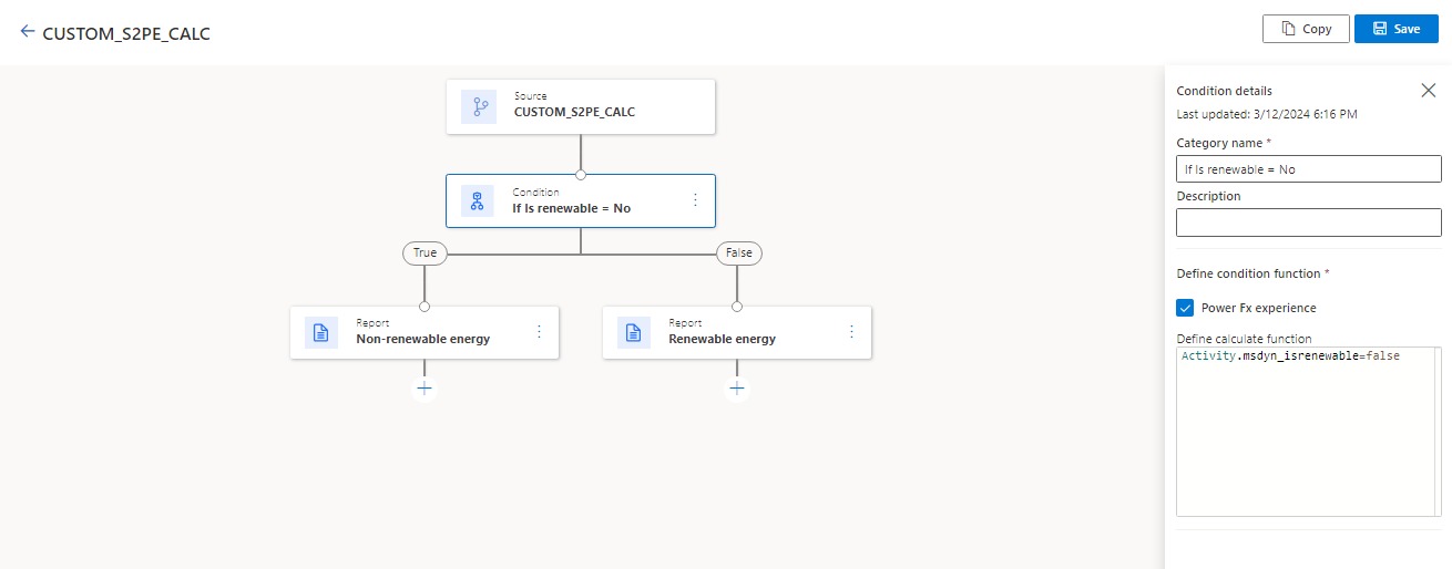
When forecasting the impact of switching from non-renewable to renewable energy, ensure that you're choosing a calculation model that supports both nonrenewable and renewable energy source calculations. The easiest way is to use a conditional on the Is renewable field.
Forecast aspects
Existing strategy: The existing strategy forecast is a view into your projected emissions if you were to change nothing about the current way you generate emissions for that category. For example, if you're forecasting the impact of switching from coal to biofuel for a particular facility, the existing strategy forecast represents the projected emissions of continuing to use coal.
New strategies: The new strategy forecast is a view into your projected emissions if you were to switch to the new business strategy represented by your forecast scenario. For example, if you're forecasting the impact of switching from coal to biofuel for a particular facility, the new strategy forecast represents the projected emissions of switching to biofuel. You can have between one and three new strategies to explore depending on how you set up your scenario.
Prediction intervals: Prediction intervals represent the estimate of an interval in which a future observation falls with a certain probability (we use 95% confidence), given the historical data. Prediction intervals essentially represent the uncertainty associated with a forecast.
Model failures and informational messages
This section explains errors or problems you might have with forecasts.
We made some adjustments in order to generate this forecast
Switching to a fallback forecasting method: We use a fallback forecasting method in case the number of historical data points and/or the data quality required to fit (S)ARIMA or ETS models is insufficient. There are two specific cases in which it becomes necessary to switch to a fallback methodology:
- Too many missing data points in an otherwise relatively uniformly spaced historical data time series
- Irregularly spaced historical data
Data uniformity check and frequency adjustment: Before forecasting, your data is aggregated on a monthly level to generate a monthly baseline and what-if forecast. However, if upon aggregation the data doesn't present a relatively uniform monthly cadence, further aggregation to two, three, four, or six months are attempted. If it isn't possible for the series to achieve relative uniformity under these adjustments, then a simpler fallback model is used for forecasting.
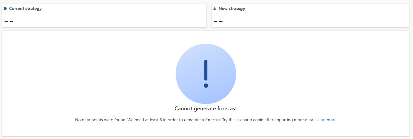
Unable to generate forecast
Historic data is too sparse: To ensure a successful forecast, we require your historical data to have a frequency of at least one data point every six months. If your data is more sparse than that interval, the forecast fails.
No or too few historical data points: The what-if analysis forecasting models require at least six data points (after frequency adjustment, described earlier in Data uniformity check and frequency adjustment) to successfully generate a forecast.
Supported time series forecasting models
Sustainability Manager supports (Seasonal) Auto Regressive Integrated Moving Average ((S)ARIMA) and Error Trend Seasonality (ETS) univariate time series forecasting models for generating forecasts on activity data. The model selection framework selects the best forecasting model based on the historical activity data. The generated activity-level forecasts go through the calculation model to transform them into emissions-level forecasts.
ARIMA and ETS are the most widely used time series forecasting methods. ETS models rely on the descriptions of trend and seasonality in the data, while ARIMA models describe the autocorrelations in the data. To learn more about these models, refer to Chapter 7 (Exponential Smoothing) and Chapter 8 (ARIMA models) of the Forecasting: Principles and Practice textbook.
On certain occasions, such as when the historical data is too little or highly irregular, a simple fallback model is selected, instead of ARIMA or ETS.


