Quantum circuit diagram conventions

Sometimes quantum algorithms are easier to understand in a circuit diagram than in the equivalent written matrix representation. This article explains how to read quantum circuit diagrams and their conventions.

For more information, see How to visualize quantum circuits diagrams.

Reading quantum circuit diagrams

In a quantum circuit, time flows from left to right. Quantum gates are ordered in chronological order with the left-most gate as the gate first applied to the qubits.

Take the following quantum circuit diagram as an example:

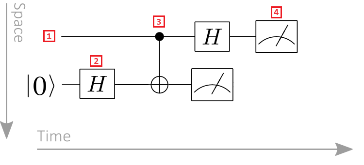
1. Qubit register: Qubit registers are displayed as horizontal lines, with each line representing a qubit. The top line is qubit register labeled 0, the second line is qubit register labeled 1, and so on.
2. Quantum gate: Quantum operations are represented by quantum gates. The term quantum gate is analogous to classical logic gates. Gates acting on one or more qubit registers are denoted as a box. In this example, the symbol represents a Hadamard operation.
3. Controlled gate: Controlled gates act on two or more qubits. In this example, the symbol represent a CNOT gate. The black circle represents the control qubit, and the cross within a circle represents the target qubit.
4. Measurement operation: The meter symbol represents a measurement operation. The measurement operation takes a qubit register as input and outputs classical information.

Applying quantum gates

Because time flows from left to right, the left-most gate is applied first For example, the action of the following quantum circuit is the unitary matrix $CBA$.

Note

Matrix multiplication obeys the opposite convention: the right-most matrix is applied first. In quantum circuit diagrams, however, the left-most gate is applied first. This difference can at times lead to confusion, so it is important to note this significant difference between the linear algebraic notation and quantum circuit diagrams.

Inputs and outputs of quantum circuits

In a quantum circuit diagram, the wires entering a quantum gate represent the qubits that are input to the quantum gate, and the wires exiting the quantum gate represent the qubits that are output from the quantum gate.

The number of inputs of a quantum gate are equal to the number of outputs of a quantum gate. This is because quantum operations are unitary and hence reversible. If a quantum gate had more outputs than inputs, it would not be reversible and hence not unitary, which is a contradiction.

For this reason any box drawn in a circuit diagram must have precisely the same number of wires entering it as exiting it.

Multi-qubit operations

Multi-qubit circuit diagrams follow similar conventions to single-qubit ones. For example, a two-qubit unitary operation $B$ can be defined to be $(H S\otimes X)$, so the equivalent quantum circuit is the following:

You can also view $B$ as having an action on a single two-qubit register rather than two one-qubit registers depending on the context in which the circuit is used.

Perhaps the most useful property of such abstract circuit diagrams is that they allow complicated quantum algorithms to be described at a high level without having to compile them down to fundamental gates. This means that you can get an intuition about the data flow for a large quantum algorithm without needing to understand all the details of how each of the subroutines within the algorithm work.

Controlled gates

Quantum controlled gates are two-qubit gates that apply a single-qubit gate to a target qubit if a control qubit is in a specific state.

For example, consider a quantum controlled gate, denoted $\Lambda(G)$, where a single qubit's value controls the application of the $G$ operation,. The controlled gate $\Lambda(G)$ can be understood by looking at the following example of a product state input:

$\Lambda(G) (\alpha \ket{0} + \beta \ket{1}) \ket{\psi} = \alpha \ket{0} \ket{\psi} + \beta \ket{1} G\ket{\psi}$

That is to say, the controlled gate applies $G$ to the register containing $\psi$ if and only if the control qubit takes the value $1$. In general, such controlled operations are described in circuit diagrams by the following symbol:

Here the black circle denotes the quantum bit on which the gate is controlled and a vertical wire denotes the unitary that is applied when the control qubit takes the value $1$.

For the special cases where $G=X$ and $G=Z$, the following notation is used to describe the controlled version of the gates (note that the controlled-X gate is the CNOT gate):

Q# provides methods to automatically generate the controlled version of an operation, which saves the programmer from having to hand code these operations. An example of this is shown below:

operation PrepareSuperposition(qubit : Qubit) : Unit
is Ctl { // Auto-generate the controlled specialization of the operation
    H(qubit);
}

Classically controlled gates

Quantum gates can also be applied after a measurement, where the result of the measurement acts as a classical control bit.

The following symbol represents a classically controlled gate, where $G$ is applied conditioned on the classical control bit being value $1$:

Measurement operator

Measurement operations take a qubit register, measures it, and outputs the result as classical information.

A measurement operation is denoted by a meter symbol and always takes as input a qubit register (denoted by a solid line) and outputs classical information (denoted by a double line). Specifically, the symbol of the measurement operation looks like:

In Q#, the Measure operator implements the measurement operation.

Example: Unitary transformation

Consider the unitary transformation $\text{ CNOT}_{01}(H\otimes 1)$. This gate sequence is of fundamental significance to quantum computing because it creates a maximally entangled two-qubit state:

$\mathrm{CNOT}_{01}(H\otimes 1)\ket{00} = \frac{1}{\sqrt{2}} \left(\ket{00} + \ket{11} \right),$

Operations with this or greater complexity are ubiquitous in quantum algorithms and quantum error correction.

The circuit diagram for preparing this maximally entangled quantum state is:

The symbol behind the Hadamard gate represents a CNOT gate, where the black circle indicates the control qubit and the cross within a circle indicates the target qubit. This quantum circuit is depicted as acting on two qubits (or equivalently two registers consisting of one qubit).

Example: Teleportation circuit diagram

Quantum teleportation is one of the best quantum algorithm for illustrating circuit components.

Quantum teleportation is a protocol that allows a quantum state to be transmitted from one qubit to another, with the help of a shared entangled state between the sender and receiver, and classical communication between them.

For learning purposes, the sender is called Alice, the receiver is called Bob, and the qubit to be teleported is called the message qubit. Alice and Bob hold one qubit each, and Alice has an extra qubit which is the message qubit.

The following circuit diagram illustrates the teleportation protocol:

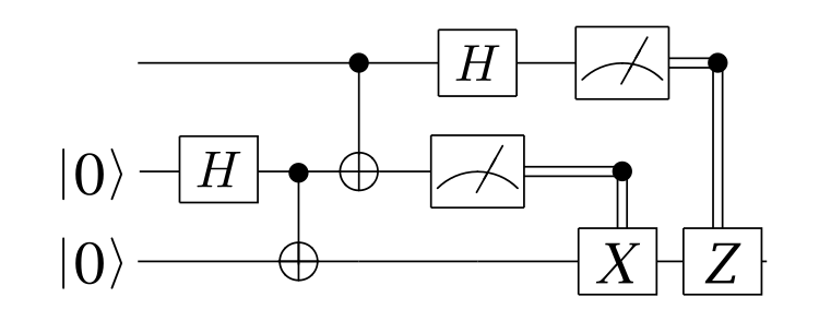
Let's break down the steps of the teleportation protocol:

1. Qubit register labeled 0 is the message qubit, qubit register labeled 1 is Alice's qubit, and qubit register labeled 2 is Bob's qubit. The message qubit is in an unknown state, and Alice and Bob's qubits are in the $\ket{0}$ state.
2. A Hadamard gate $H$ is applied to Alice's qubit. Because the qubit is in the $\ket{0}$ state, the resulting state is $\frac{1}{\sqrt{2}}(\ket{0} + \ket{1})$.
3. A CNOT gate is applied to Alice and Bob's qubits. Alice's qubit is the control qubit, and Bob's qubit is the target qubit. The resulting state is $\frac{1}{\sqrt{2}}(\ket{00} + \ket{11})$. Alice and Bob now share an entangled state.
4. A CNOT gate is applied to the message qubit and Alice's qubit. Since Alice's qubit is also entangled with Bob's qubit, the resulting state is a three-qubit entangled state.
5. A Hadamard gate $H$ is applied to the message qubit.
6. Alice measures her two qubits and communicates the measurement results to Bob - this isn't reflected in the circuit. The measurement results are two classical bits, which can take the values 00, 01, 10, or 1
7. Two classically controlled Pauli gates are applied to Bob's qubit, depending on the result bit being value $1$. The resulting state is the original message qubit state.

Next steps

• Quantum oracles
• Grover's algorithm
• Quantum Intermediate Representation
• Vectors and matrices