Kusto Query Language in Microsoft Sentinel
Kusto Query Language is the language you will use to work with and manipulate data in Microsoft Sentinel. The logs you feed into your workspace aren't worth much if you can't analyze them and get the important information hidden in all that data. Kusto Query Language has not only the power and flexibility to get that information, but the simplicity to help you get started quickly. If you have a background in scripting or working with databases, a lot of the content of this article will feel very familiar. If not, don't worry, as the intuitive nature of the language quickly enables you to start writing your own queries and driving value for your organization.
This article introduces the basics of Kusto Query Language, covering some of the most used functions and operators, which should address 75 to 80 percent of the queries you will write day to day. When you'll need more depth, or to run more advanced queries, you can take advantage of the new Advanced KQL for Microsoft Sentinel workbook (see this introductory blog post). See also the official Kusto Query Language documentation as well as a variety of online courses (such as Pluralsight's).
Background - Why Kusto Query Language?
Microsoft Sentinel is built on top of the Azure Monitor service and it uses Azure Monitor’s Log Analytics workspaces to store all of its data. This data includes any of the following:
- data ingested from external sources into predefined tables using Microsoft Sentinel data connectors.
- data ingested from external sources into user-defined custom tables, using custom-created data connectors as well as some types of out-of-the-box connectors.
- data created by Microsoft Sentinel itself, resulting from the analyses it creates and performs - for example, alerts, incidents, and UEBA-related information.
- data uploaded to Microsoft Sentinel to assist with detection and analysis - for example, threat intelligence feeds and watchlists.
Kusto Query Language was developed as part of the Azure Data Explorer service, and it’s therefore optimized for searching through big-data stores in a cloud environment. Inspired by famed undersea explorer Jacques Cousteau (and pronounced accordingly "koo-STOH"), it’s designed to help you dive deep into your oceans of data and explore their hidden treasures.
Kusto Query Language is also used in Azure Monitor (and therefore in Microsoft Sentinel), including some additional Azure Monitor features, which allow you to retrieve, visualize, analyze, and parse data in Log Analytics data stores. In Microsoft Sentinel, you're using tools based on Kusto Query Language whenever you’re visualizing and analyzing data and hunting for threats, whether in existing rules and workbooks, or in building your own.
Because Kusto Query Language is a part of nearly everything you do in Microsoft Sentinel, a clear understanding of how it works helps you get that much more out of your SIEM.
What is a query?
A Kusto Query Language query is a read-only request to process data and return results – it doesn’t write any data. Queries operate on data that's organized into a hierarchy of databases, tables, and columns, similar to SQL.
Requests are stated in plain language and use a data-flow model designed to make the syntax easy to read, write, and automate. We'll see this in detail.
Kusto Query Language queries are made up of statements separated by semicolons. There are many kinds of statements, but only two widely used types that we’ll discuss here:
tabular expression statements are what we typically mean when we talk about queries – these are the actual body of the query. The important thing to know about tabular expression statements is that they accept a tabular input (a table or another tabular expression) and produce a tabular output. At least one of these is required. Most of the rest of this article will discuss this kind of statement.
let statements allow you to create and define variables and constants outside the body of the query, for easier readability and versatility. These are optional and depend on your particular needs. We'll address this kind of statement at the end of the article.
Demo environment
You can practice Kusto Query Language statements - including the ones in this article - in a Log Analytics demo environment in the Azure portal. There is no charge to use this practice environment, but you do need an Azure account to access it.
Explore the demo environment. Like Log Analytics in your production environment, it can be used in a number of ways:
Choose a table on which to build a query. From the default Tables tab (shown in the red rectangle at the upper left), select a table from the list of tables grouped by topics (shown at the lower left). Expand the topics to see the individual tables, and you can further expand each table to see all its fields (columns). Double-clicking on a table or a field name will place it at the point of the cursor in the query window. Type the rest of your query following the table name, as directed below.
Find an existing query to study or modify. Select the Queries tab (shown in the red rectangle at the upper left) to see a list of queries available out-of-the-box. Or, select Queries from the button bar at the top right. You can explore the queries that come with Microsoft Sentinel out-of-the-box. Double-clicking a query will place the whole query in the query window at the point of the cursor.
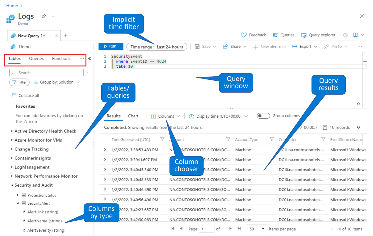
Like in this demo environment, you can query and filter data in the Microsoft Sentinel Logs page. You can select a table and drill down to see columns. You can modify the default columns shown using the Column chooser, and you can set the default time range for queries. If the time range is explicitly defined in the query, the time filter will be unavailable (grayed out).
Query structure
A good place to start learning Kusto Query Language is to understand the overall query structure. The first thing you'll notice when looking at a Kusto query is the use of the pipe symbol (|). The structure of a Kusto query starts with getting your data from a data source and then passing the data across a "pipeline," and each step provides some level of processing and then passes the data to the next step. At the end of the pipeline, you will get your final result. In effect, this is our pipeline:
Get Data | Filter | Summarize | Sort | Select
This concept of passing data down the pipeline makes for a very intuitive structure, as it is easy to create a mental picture of your data at each step.
To illustrate this, let's take a look at the following query, which looks at Microsoft Entra sign-in logs. As you read through each line, you can see the keywords that indicate what's happening to the data. We've included the relevant stage in the pipeline as a comment in each line.
Note
You can add comments to any line in a query by preceding them with a double slash (//).
SigninLogs                              // Get data
| evaluate bag_unpack(LocationDetails)  // Ignore this line for now; we'll come back to it at the end.
| where RiskLevelDuringSignIn == 'none' // Filter
   and TimeGenerated >= ago(7d)         // Filter
| summarize Count = count() by city     // Summarize
| sort by Count desc                    // Sort
| take 5                                // Select
Because the output of every step serves as the input for the following step, the order of the steps can determine the query's results and affect its performance. It's crucial that you order the steps according to what you want to get out of the query.
Tip
- A good rule of thumb is to filter your data early, so you are only passing relevant data down the pipeline. This will greatly increase performance and ensure that you aren't accidentally including irrelevant data in summarization steps.
- This article will point out some other best practices to keep in mind. For a more complete list, see query best practices.
Hopefully, you now have an appreciation for the overall structure of a query in Kusto Query Language. Now let's look at the actual query operators themselves, which are used to create a query.
Data types
Before we get into the query operators, let's first take a quick look at data types. As in most languages, the data type determines what calculations and manipulations can be run against a value. For example, if you have a value that is of type string, you won't be able to perform arithmetic calculations against it.
In Kusto Query Language, most of the data types follow standard conventions and have names you've probably seen before. The following table shows the full list:
Data type table
| Type | Additional name(s) | Equivalent .NET type |
|---|---|---|
bool |
Boolean |
System.Boolean |
datetime |
Date |
System.DateTime |
dynamic |
System.Object |
|
guid |
uuid, uniqueid |
System.Guid |
int |
System.Int32 |
|
long |
System.Int64 |
|
real |
Double |
System.Double |
string |
System.String |
|
timespan |
Time |
System.TimeSpan |
decimal |
System.Data.SqlTypes.SqlDecimal |
While most of the data types are standard, you might be less familiar with types like dynamic, timespan, and guid.
Dynamic has a structure very similar to JSON, but with one key difference: It can store Kusto Query Language-specific data types that traditional JSON cannot, such as a nested dynamic value, or timespan. Here's an example of a dynamic type:
{
"countryOrRegion":"US",
"geoCoordinates": {
"longitude":-122.12094116210936,
"latitude":47.68050003051758
},
"state":"Washington",
"city":"Redmond"
}
Timespan is a data type that refers to a measure of time such as hours, days, or seconds. Do not confuse timespan with datetime, which evaluates to an actual date and time, not a measure of time. The following table shows a list of timespan suffixes.
Timespan suffixes
| Function | Description |
|---|---|
D |
days |
H |
hours |
M |
minutes |
S |
seconds |
Ms |
milliseconds |
Microsecond |
microseconds |
Tick |
nanoseconds |
Guid is a datatype representing a 128-bit, globally-unique identifier, which follows the standard format of [8]-[4]-[4]-[4]-[12], where each [number] represents the number of characters and each character can range from 0-9 or a-f.
Note
Kusto Query Language has both tabular and scalar operators. Throughout the rest of this article, if you simply see the word "operator," you can assume it means tabular operator, unless otherwise noted.
Getting, limiting, sorting, and filtering data
The core vocabulary of Kusto Query Language - the foundation that will allow you to accomplish the overwhelming majority of your tasks - is a collection of operators for filtering, sorting, and selecting your data. The remaining tasks you will need to do will require you to stretch your knowledge of the language to meet your more advanced needs. Let's expand a bit on some of the commands we used in our above example and look at take, sort, and where.
For each of these operators, we'll examine its use in our previous SigninLogs example, and learn either a useful tip or a best practice.
Getting data
The first line of any basic query specifies which table you want to work with. In the case of Microsoft Sentinel, this will likely be the name of a log type in your workspace, such as SigninLogs, SecurityAlert, or CommonSecurityLog. For example:
SigninLogs
Note that in Kusto Query Language, log names are case sensitive, so SigninLogs and signinLogs will be interpreted differently. Take care when choosing names for your custom logs, so they are easily identifiable and not too similar to another log.
Limiting data: take / limit
The take operator (and the identical limit operator) is used to limit your results by returning only a given number of rows. It's followed by an integer that specifies the number of rows to return. Typically, it's used at the end of a query after you have determined your sort order, and in such a case it will return the given number of rows at the top of the sorted order.
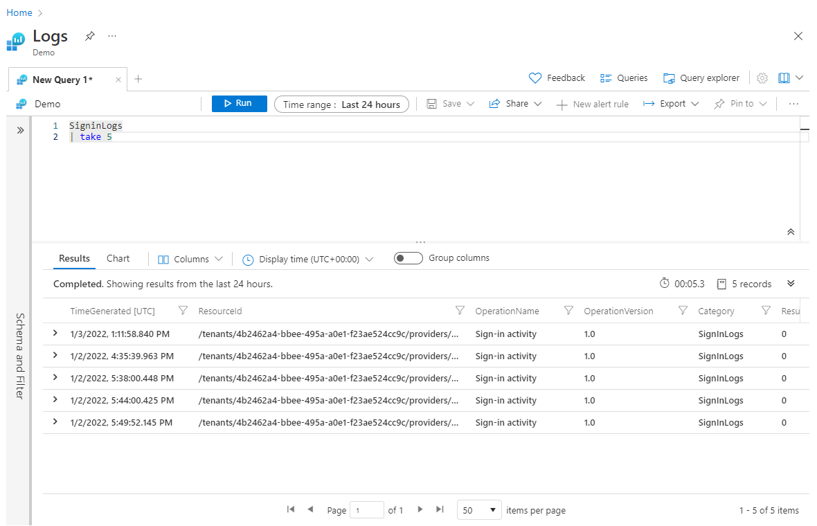
Using take earlier in the query can be useful for testing a query, when you don't want to return large datasets. However, if you place the take operation before any sort operations, take will return rows selected at random - and possibly a different set of rows every time the query is run. Here's an example of using take:
SigninLogs
      | take 5
Tip
When working on a brand-new query where you may not know what the query will look like, it can be useful to put a take statement at the beginning to artificially limit your dataset for faster processing and experimentation. Once you are happy with the full query, you can remove the initial take step.
Sorting data: sort / order
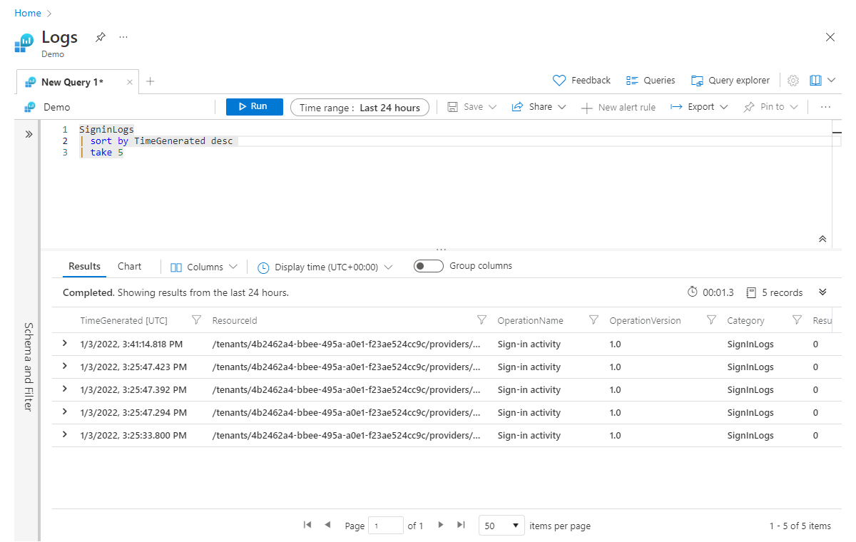
The sort operator (and the identical order operator) is used to sort your data by a specified column. In the following example, we ordered the results by TimeGenerated and set the order direction to descending with the desc parameter, placing the highest values first; for ascending order we would use asc.
Note
The default direction for sorts is descending, so technically you only have to specify if you want to sort in ascending order. However, specifying the sort direction in any case will make your query more readable.
SigninLogs
| sort by TimeGenerated desc
| take 5
As we mentioned, we put the sort operator before the take operator. We need to sort first to make sure we get the appropriate five records.
Top
The top operator allows us to combine the sort and take operations into a single operator:
SigninLogs
| top 5 by TimeGenerated desc
In cases where two or more records have the same value in the column you are sorting by, you can add more columns to sort by. Add extra sorting columns in a comma-separated list, located after the first sorting column, but before the sort order keyword. For example:
SigninLogs
| sort by TimeGenerated, Identity desc
| take 5
Now, if TimeGenerated is the same between multiple records, it will then try to sort by the value in the Identity column.
Note
When to use sort and take, and when to use top
If you're only sorting on one field, use
top, as it provides better performance than the combination ofsortandtake.If you need to sort on more than one field (like in the last example above),
topcan't do that, so you must usesortandtake.
Filtering data: where
The where operator is arguably the most important operator, because it's the key to making sure you are only working with the subset of data that is relevant to your scenario. You should do your best to filter your data as early in the query as possible because doing so will improve query performance by reducing the amount of data that needs to be processed in subsequent steps; it also ensures that you are only performing calculations on the desired data. See this example:
SigninLogs
| where TimeGenerated >= ago(7d)
| sort by TimeGenerated, Identity desc
| take 5
The where operator specifies a variable, a comparison (scalar) operator, and a value. In our case, we used >= to denote that the value in the TimeGenerated column needs to be greater than (that is, later than) or equal to seven days ago.
There are two types of comparison operators in Kusto Query Language: string and numerical. The following table shows the full list of numerical operators:
Numerical operators
| Operator | Description |
|---|---|
+ |
Addition |
- |
Subtraction |
* |
Multiplication |
/ |
Division |
% |
Modulo |
< |
Less than |
> |
Greater than |
== |
Equal to |
!= |
Not equal to |
<= |
Less than or equal to |
>= |
Greater than or equal to |
in |
Equal to one of the elements |
!in |
Not equal to any of the elements |
The list of string operators is a much longer list because it has permutations for case sensitivity, substring locations, prefixes, suffixes, and much more. The == operator is both a numeric and string operator, meaning it can be used for both numbers and text. For example, both of the following statements would be valid where statements:
| where ResultType == 0| where Category == 'SignInLogs'
Tip
Best Practice: In most cases, you will probably want to filter your data by more than one column, or filter the same column in more than one way. In these instances, there are two best practices you should keep in mind.
You can combine multiple where statements into a single step by using the and keyword. For example:
SigninLogs
| where Resource == ResourceGroup
    and TimeGenerated >= ago(7d)
When you have multiple filters joined into a single where statement using the and keyword, like above, you will get better performance by putting filters that only reference a single column first. So, a better way to write the above query would be:
SigninLogs
| where TimeGenerated >= ago(7d)
    and Resource == ResourceGroup
In this example, the first filter mentions a single column (TimeGenerated), while the second references two columns (Resource and ResourceGroup).
Summarizing data
Summarize is one of the most important tabular operators in Kusto Query Language, but it also is one of the more complex operators to learn if you are new to query languages in general. The job of summarize is to take in a table of data and output a new table that is aggregated by one or more columns.
Structure of the summarize statement
The basic structure of a summarize statement is as follows:
| summarize <aggregation> by <column>
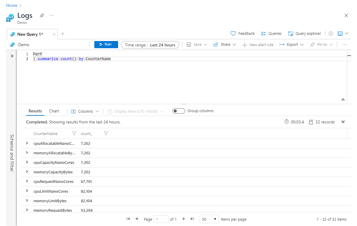
For example, the following would return the count of records for each CounterName value in the Perf table:
Perf
| summarize count() by CounterName
Because the output of summarize is a new table, any columns not explicitly specified in the summarize statement will not be passed down the pipeline. To illustrate this concept, consider this example:
Perf
| project ObjectName, CounterValue, CounterName
| summarize count() by CounterName
| sort by ObjectName asc
On the second line, we are specifying that we only care about the columns ObjectName, CounterValue, and CounterName. We then summarized to get the record count by CounterName and finally, we attempt to sort the data in ascending order based on the ObjectName column. Unfortunately, this query will fail with an error (indicating that the ObjectName is unknown) because when we summarized, we only included the Count and CounterName columns in our new table. To avoid this error, we can simply add ObjectName to the end of our summarize step, like this:
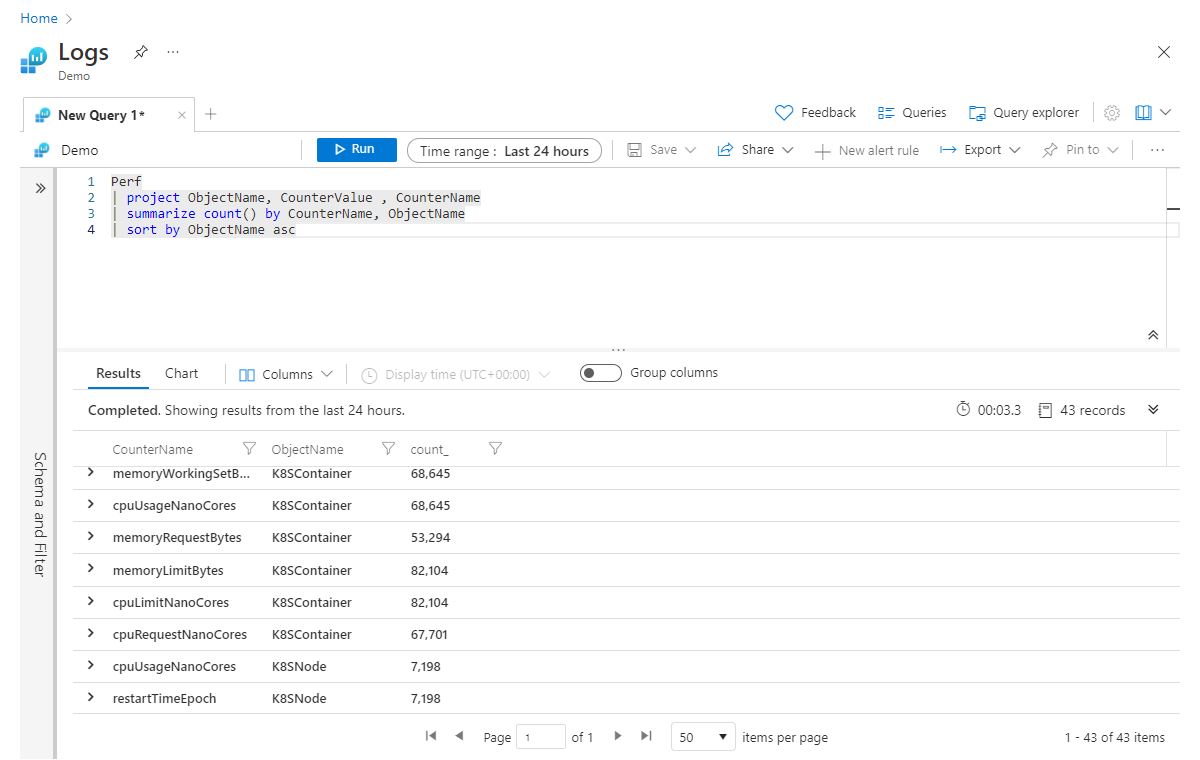
Perf
| project ObjectName, CounterValue , CounterName
| summarize count() by CounterName, ObjectName
| sort by ObjectName asc
The way to read the summarize line in your head would be: "summarize the count of records by CounterName, and group by ObjectName". You can continue adding columns, separated by commas, to the end of the summarize statement.
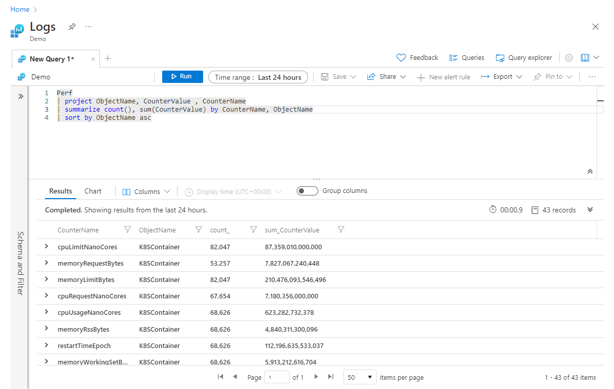
Building on the previous example, if we want to aggregate multiple columns at the same time, we can achieve this by adding aggregations to the summarize operator, separated by commas. In the example below, we are getting not only a count of all the records but also a sum of the values in the CounterValue column across all records (that match any filters in the query):
Perf
| project ObjectName, CounterValue , CounterName
| summarize count(), sum(CounterValue) by CounterName, ObjectName
| sort by ObjectName asc
Renaming aggregated columns
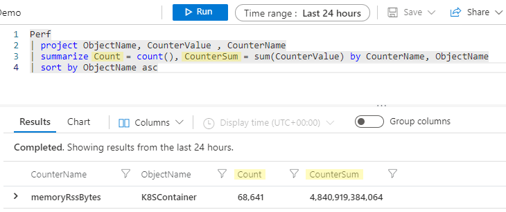
This seems like a good time to talk about column names for these aggregated columns. At the start of this section, we said the summarize operator takes in a table of data and produces a new table, and only the columns you specify in the summarize statement will continue down the pipeline. Therefore, if you were to run the above example, the resulting columns for our aggregation would be count_ and sum_CounterValue.
The Kusto engine will automatically create a column name without us having to be explicit, but often, you will find that you will prefer your new column have a friendlier name. You can easily rename your column in the summarize statement by specifying a new name, followed by = and the aggregation, like so:
Perf
| project ObjectName, CounterValue , CounterName
| summarize Count = count(), CounterSum = sum(CounterValue) by CounterName, ObjectName
| sort by ObjectName asc
Now, our summarized columns will be named Count and CounterSum.
There is much more to the summarize operator than we can cover here, but you should invest the time to learn it because it is a key component to any data analysis you plan to perform on your Microsoft Sentinel data.
Aggregation reference
The are many aggregation functions, but some of the most commonly used are sum(), count(), and avg(). Here's a partial list (see the full list):
Aggregation functions
| Function | Description |
|---|---|
arg_max() |
Returns one or more expressions when argument is maximized |
arg_min() |
Returns one or more expressions when argument is minimized |
avg() |
Returns average value across the group |
buildschema() |
Returns the minimal schema that admits all values of the dynamic input |
count() |
Returns count of the group |
countif() |
Returns count with the predicate of the group |
dcount() |
Returns approximate distinct count of the group elements |
make_bag() |
Returns a property bag of dynamic values within the group |
make_list() |
Returns a list of all the values within the group |
make_set() |
Returns a set of distinct values within the group |
max() |
Returns the maximum value across the group |
min() |
Returns the minimum value across the group |
percentiles() |
Returns the percentile approximate of the group |
stdev() |
Returns the standard deviation across the group |
sum() |
Returns the sum of the elements within the group |
take_any() |
Returns random non-empty value for the group |
variance() |
Returns the variance across the group |
Selecting: adding and removing columns
As you start working more with queries, you may find that you have more information than you need on your subjects (that is, too many columns in your table). Or you might need more information than you have (that is, you need to add a new column that will contain the results of analysis of other columns). Let's look at a few of the key operators for column manipulation.
Project and project-away
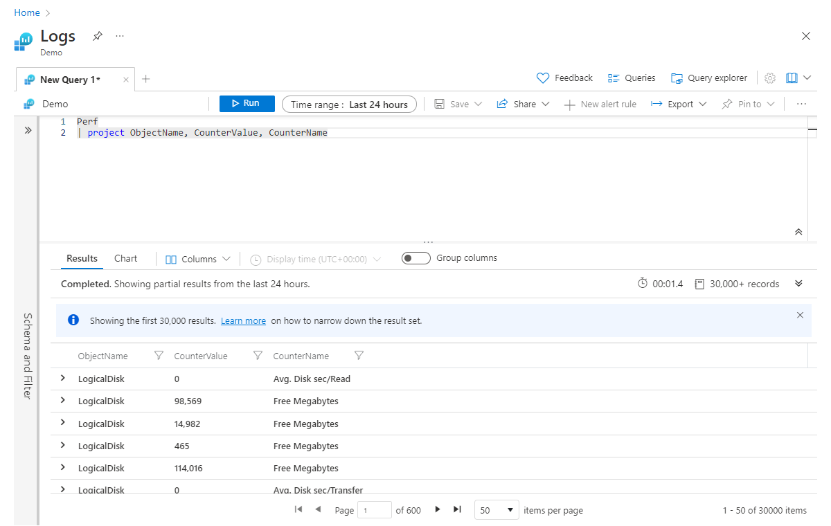
Project is roughly equivalent to many languages' select statements. It allows you to choose which columns to keep. The order of the columns returned will match the order of the columns you list in your project statement, as shown in this example:
Perf
| project ObjectName, CounterValue, CounterName
As you can imagine, when you are working with very wide datasets, you may have lots of columns you want to keep, and specifying them all by name would require a lot of typing. For those cases, you have project-away, which lets you specify which columns to remove, rather than which ones to keep, like so:
Perf
| project-away MG, _ResourceId, Type
Tip
It can be useful to use project in two locations in your queries, at the beginning and again at the end. Using project early in your query can help improve performance by stripping away large chunks of data you don't need to pass down the pipeline. Using it again at the end lets you get rid of any columns that may have been created in previous steps and aren't needed in your final output.
Extend
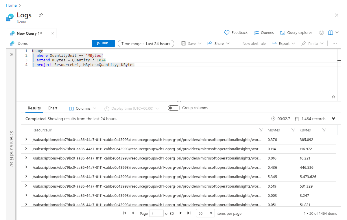
Extend is used to create a new calculated column. This can be useful when you want to perform a calculation against existing columns and see the output for every row. Let's look at a simple example where we calculate a new column called Kbytes, which we can calculate by multiplying the MB value (in the existing Quantity column) by 1,024.
Usage
| where QuantityUnit == 'MBytes'
| extend KBytes = Quantity * 1024
| project ResourceUri, MBytes=Quantity, KBytes
On the final line in our project statement, we renamed the Quantity column to Mbytes, so we can easily tell which unit of measure is relevant to each column.
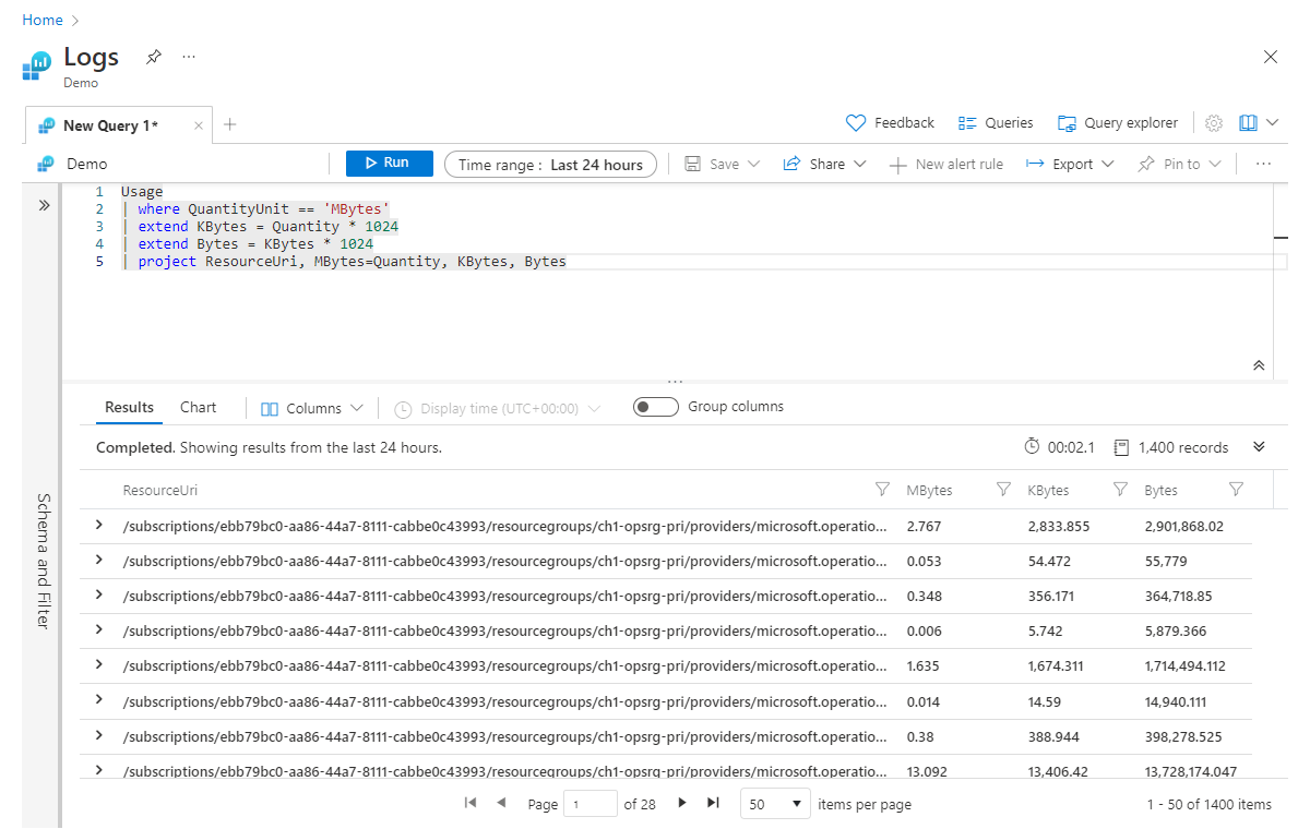
It's worth noting that extend also works with already calculated columns. For example, we can add one more column called Bytes that is calculated from Kbytes:
Usage
| where QuantityUnit == 'MBytes'
| extend KBytes = Quantity * 1024
| extend Bytes = KBytes * 1024
| project ResourceUri, MBytes=Quantity, KBytes, Bytes
Joining tables
Much of your work in Microsoft Sentinel can be carried out by using a single log type, but there are times when you will want to correlate data together or perform a lookup against another set of data. Like most query languages, Kusto Query Language offers a few operators used to perform various types of joins. In this section, we will look at the most-used operators, union and join.
Union
Union simply takes two or more tables and returns all the rows. For example:
OfficeActivity
| union SecurityEvent
This would return all rows from both the OfficeActivity and SecurityEvent tables. Union offers a few parameters that can be used to adjust how the union behaves. Two of the most useful are withsource and kind:
OfficeActivity
| union withsource = SourceTable kind = inner SecurityEvent
The withsource parameter lets you specify the name of a new column whose value in a given row will be the name of the table from which the row came. In the example above, we named the column SourceTable, and depending on the row, the value will either be OfficeActivity or SecurityEvent.
The other parameter we specified was kind, which has two options: inner or outer. In the example above, we specified inner, which means the only columns that will be kept during the union are those that exist in both tables. Alternatively, if we had specified outer (which is the default value), then all columns from both tables would be returned.
Join
Join works similarly to union, except instead of joining tables to make a new table, we are joining rows to make a new table. Like most database languages, there are multiple types of joins you can perform. The general syntax for a join is:
T1
| join kind = <join type>
(
               T2
) on $left.<T1Column> == $right.<T2Column>
After the join operator, we specify the kind of join we want to perform followed by an open parenthesis. Within the parentheses is where you specify the table you want to join, as well as any other query statements on that table you wish to add. After the closing parenthesis, we use the on keyword followed by our left ($left.<columnName> keyword) and right ($right.<columnName>) columns separated with the == operator. Here's an example of an inner join:
OfficeActivity
| where TimeGenerated >= ago(1d)
    and LogonUserSid != ''
| join kind = inner (
    SecurityEvent
    | where TimeGenerated >= ago(1d)
        and SubjectUserSid != ''
) on $left.LogonUserSid == $right.SubjectUserSid
Note
If both tables have the same name for the columns on which you are performing a join, you don't need to use $left and $right; instead, you can just specify the column name. Using $left and $right, however, is more explicit and generally considered to be a good practice.
For your reference, the following table shows a list of available types of joins.
Types of Joins
| Join Type | Description |
|---|---|
inner |
Returns a single for each combination of matching rows from both tables. |
innerunique |
Returns rows from the left table with distinct values in linked field that have a match in the right table. This is the default unspecified join type. |
leftsemi |
Returns all records from the left table that have a match in the right table. Only columns from the left table will be returned. |
rightsemi |
Returns all records from the right table that have a match in the left table. Only columns from the right table will be returned. |
leftanti/leftantisemi |
Returns all records from the left table that don't have a match in the right table. Only columns from the left table will be returned. |
rightanti/rightantisemi |
Returns all records from the right table that don't have a match in the left table. Only columns from the right table will be returned. |
leftouter |
Returns all records from the left table. For records that have no match in the right table, cell values will be null. |
rightouter |
Returns all records from the right table. For records that have no match in the left table, cell values will be null. |
fullouter |
Returns all records from both left and right tables, matching or not. Unmatched values will be null. |
Tip
It's a best practice to have your smallest table on the left. In some cases, following this rule can give you huge performance benefits, depending on the types of joins you are performing and the size of the tables.
Evaluate
You may remember that back in the first example, we saw the evaluate operator on one of the lines. The evaluate operator is less commonly used than the ones we have touched on previously. However, knowing how the evaluate operator works is well worth your time. Once more, here is that first query, where you will see evaluate on the second line.
SigninLogs
| evaluate bag_unpack(LocationDetails)
| where RiskLevelDuringSignIn == 'none'
   and TimeGenerated >= ago(7d)
| summarize Count = count() by city
| sort by Count desc
| take 5
This operator allows you to invoke available plugins (basically built-in functions). Many of these plugins are focused around data science, such as autocluster, diffpatterns, and sequence_detect, allowing you to perform advanced analysis and discover statistical anomalies and outliers.
The plugin used in the above example was called bag_unpack, and it makes it very easy to take a chunk of dynamic data and convert it to columns. Remember, dynamic data is a data type that looks very similar to JSON, as shown in this example:
{
"countryOrRegion":"US",
"geoCoordinates": {
"longitude":-122.12094116210936,
"latitude":47.68050003051758
},
"state":"Washington",
"city":"Redmond"
}
In this case, we wanted to summarize the data by city, but city is contained as a property within the LocationDetails column. To use the city property in our query, we had to first convert it to a column using bag_unpack.
Going back to our original pipeline steps, we saw this:
Get Data | Filter | Summarize | Sort | Select
Now that we've considered the evaluate operator, we can see that it represents a new stage in the pipeline, which now looks like this:
Get Data | Parse | Filter | Summarize | Sort | Select
There are many other examples of operators and functions that can be used to parse data sources into a more readable and manipulatable format. You can learn about them - and the rest of the Kusto Query Language - in the full documentation and in the workbook.
Let statements
Now that we've covered many of the major operators and data types, let's wrap up with the let statement, which is a great way to make your queries easier to read, edit, and maintain.
Let allows you to create and set a variable, or to assign a name to an expression. This expression could be a single value, but it could also be a whole query. Here's a simple example:
let aWeekAgo = ago(7d);
SigninLogs
| where TimeGenerated >= aWeekAgo
Here, we specified a name of aWeekAgo and set it to be equal to the output of a timespan function, which returns a datetime value. We then terminate the let statement with a semicolon. Now we have a new variable called aWeekAgo that can be used anywhere in our query.
As we just mentioned, you can use a let statement to take a whole query and give the result a name. Since query results, being tabular expressions, can be used as the inputs of queries, you can treat this named result as a table for the purposes of running another query on it. Here's a slight modification to the previous example:
let aWeekAgo = ago(7d);
let getSignins = SigninLogs
| where TimeGenerated >= aWeekAgo;
getSignins
In this case, we created a second let statement, where we wrapped our whole query into a new variable called getSignins. Just like before, we terminate the second let statement with a semicolon. Then we call the variable on the final line, which will run the query. Notice that we were able to use aWeekAgo in the second let statement. This is because we specified it on the previous line; if we were to swap the let statements so that getSignins came first, we would get an error.
Now we can use getSignins as the basis of another query (in the same window):
let aWeekAgo = ago(7d);
let getSignins = SigninLogs
| where TimeGenerated >= aWeekAgo;
getSignins
| where level >= 3
| project IPAddress, UserDisplayName, Level
Let statements give you more power and flexibility in helping to organize your queries. Let can define scalar and tabular values as well as create user-defined functions. They truly come in handy when you are organizing more complex queries that may be doing multiple joins.
Next steps
While this article has barely scratched the surface, you've now got the necessary foundation, and we've covered the parts you'll be using most often to get your work done in Microsoft Sentinel.
Advanced KQL for Microsoft Sentinel workbook
Take advantage of a Kusto Query Language workbook right in Microsoft Sentinel itself - the Advanced KQL for Microsoft Sentinel workbook. It gives you step-by-step help and examples for many of the situations you're likely to encounter during your day-to-day security operations, and also points you to lots of ready-made, out-of-the-box examples of analytics rules, workbooks, hunting rules, and more elements that use Kusto queries. Launch this workbook from the Workbooks blade in Microsoft Sentinel.
Advanced KQL Framework Workbook - Empowering you to become KQL-savvy is an excellent blog post that shows you how to use this workbook.
More resources
See this collection of learning, training, and skilling resources for broadening and deepening your knowledge of Kusto Query Language.