Migrating Time Series Insights (TSI) Gen2 to Azure Data Explorer

Article
10/05/2022

Note

The Time Series Insights (TSI) service will no longer be supported after March 2025. Consider migrating existing TSI environments to alternative solutions as soon as possible. For more information on the deprecation and migration, visit our documentation.

Overview

High-level migration recommendations.

Feature	Gen2 State	Migration Recommended
Ingesting JSON from Hub with flattening and escaping	TSI Ingestion	ADX - OneClick Ingest / Wizard
Open Cold store	Customer Storage Account	Continuous data export to customer specified external table in ADLS.
PBI Connector	Private Preview	Use ADX PBI Connector. Rewrite TSQ to KQL manually.
Spark Connector	Private Preview. Query telemetry data. Query model data.	Migrate data to ADX. Use ADX Spark connector for telemetry data + export model to JSON and load in Spark. Rewrite queries in KQL.
Bulk Upload	Private Preview	Use ADX OneClick Ingest and LightIngest. An optionally, set up partitioning within ADX.
Time Series Model		Can be exported as JSON file. Can be imported to ADX to perform joins in KQL.
TSI Explorer	Toggling warm and cold	ADX Dashboards
Query language	Time Series Queries (TSQ)	Rewrite queries in KQL. Use Kusto SDKs instead of TSI ones.

Migrating Telemetry

Use PT=Time folder in the storage account to retrieve the copy of all telemetry in the environment. For more information, please see Data Storage.

Migration Step 1 – Get Statistics about Telemetry Data

Data

Env overview
- Record Environment ID from first part of Data Access FQDN (for example, d390b0b0-1445-4c0c-8365-68d6382c1c2a From .env.crystal-dev.windows-int.net)
Env Overview -> Storage Configuration -> Storage Account
Use Storage Explorer to get folder statistics
- Record size and the number of blobs of PT=Time folder. For customers in private preview of Bulk Import, also record PT=Import size and number of blobs.

Migration Step 2 – Migrate Telemetry To ADX

Create ADX cluster

Define the cluster size based on data size using the ADX Cost Estimator.
1. From Event Hubs (or IoT Hub) metrics, retrieve the rate of how much data it's ingested per day. From the Storage Account connected to the TSI environment, retrieve how much data there is in the blob container used by TSI. This information will be used to compute the ideal size of an ADX Cluster for your environment.
2. Open the Azure Data Explorer Cost Estimator and fill the existing fields with the information found. Set “Workload type” as “Storage Optimized”, and "Hot Data" with the total amount of data queried actively.
3. After providing all the information, Azure Data Explorer Cost Estimator will suggest a VM size and number of instances for your cluster. Analyze if the size of actively queried data will fit in the Hot Cache. Multiply the number of instances suggested by the cache size of the VM size, per example:
  - Cost Estimator suggestion: 9x DS14 + 4 TB (cache)
  - Total Hot Cache suggested: 36 TB = [9x (instances) x 4 TB (of Hot Cache per node)]
4. More factors to consider:
  - Environment growth: when planning the ADX Cluster size consider the data growth along the time.
  - Hydration and Partitioning: when defining the number of instances in ADX Cluster, consider extra nodes (by 2-3x) to speed up hydration and partitioning.
  - For more information about compute selection, see Select the correct compute SKU for your Azure Data Explorer cluster.
To best monitor your cluster and the data ingestion, you should enable Diagnostic Settings and send the data to a Log Analytics Workspace.
1. In the Azure Data Explorer blade, go to “Monitoring | Diagnostic settings” and click on “Add diagnostic setting”
2. Fill in the following
  1. Diagnostic setting name: Display Name for this configuration
  2. Logs: At minimum select SucceededIngestion, FailedIngestion, IngestionBatching
  3. Select the Log Analytics Workspace to send the data to (if you don’t have one you’ll need to provision one before this step)
Data partitioning.
1. For most data sets, the default ADX partitioning is enough.
2. Data partitioning is beneficial in a very specific set of scenarios, and shouldn't be applied otherwise:
  1. Improving query latency in big data sets where most queries filter on a high cardinality string column, e.g. a time-series ID.
  2. When ingesting out-of-order data, e.g. when events from the past may be ingested days or weeks after their generation in the origin.
3. For more information, check ADX Data Partitioning Policy.

Prepare for Data Ingestion

Go to https://dataexplorer.azure.com.
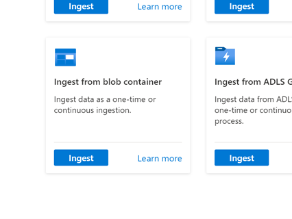
Go to Data tab and select ‘Ingest from blob container’
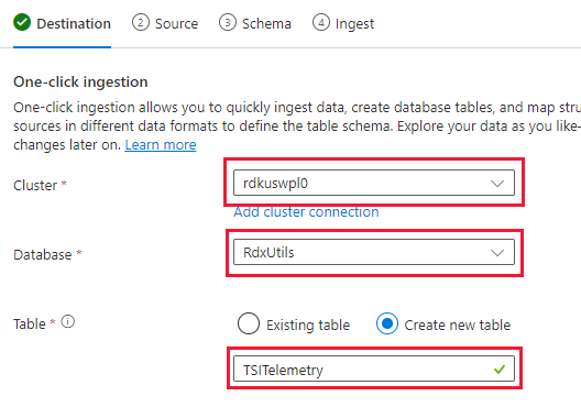
Select Cluster, Database, and create a new Table with the name you choose for the TSI data
Select Next: Source
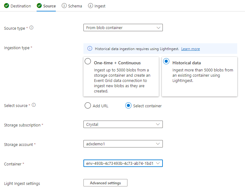
In the Source tab select:
1. Historical data
2. “Select Container”
3. Choose the Subscription and Storage account for your TSI data
4. Choose the container that correlates to your TSI Environment
Select on Advanced settings
1. Creation time pattern: '/'yyyyMMddHHmmssfff'_'
2. Blob name pattern: *.parquet
3. Select on “Don’t wait for ingestion to complete”
Under File Filters, add the Folder path V=1/PT=Time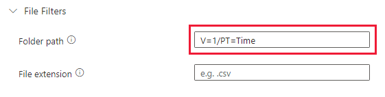
Select Next: Schema

Note

TSI applies some flattening and escaping when persisting columns in Parquet files. See these links for more details: flattening and escaping rules, ingestion rules updates.

If schema is unknown or varying
1. Remove all columns that are infrequently queried, leaving at least timestamp and TSID column(s).
2. Add new column of dynamic type and map it to the whole record using $ path.
  
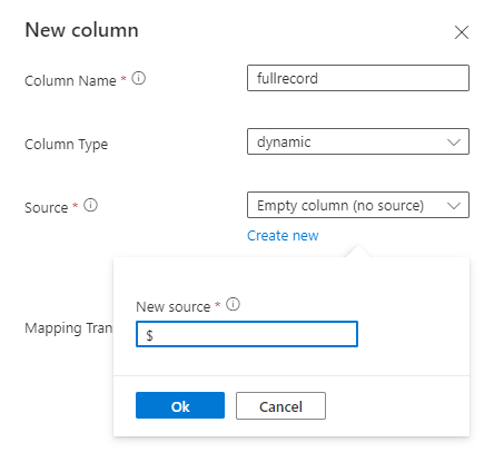
  Example:
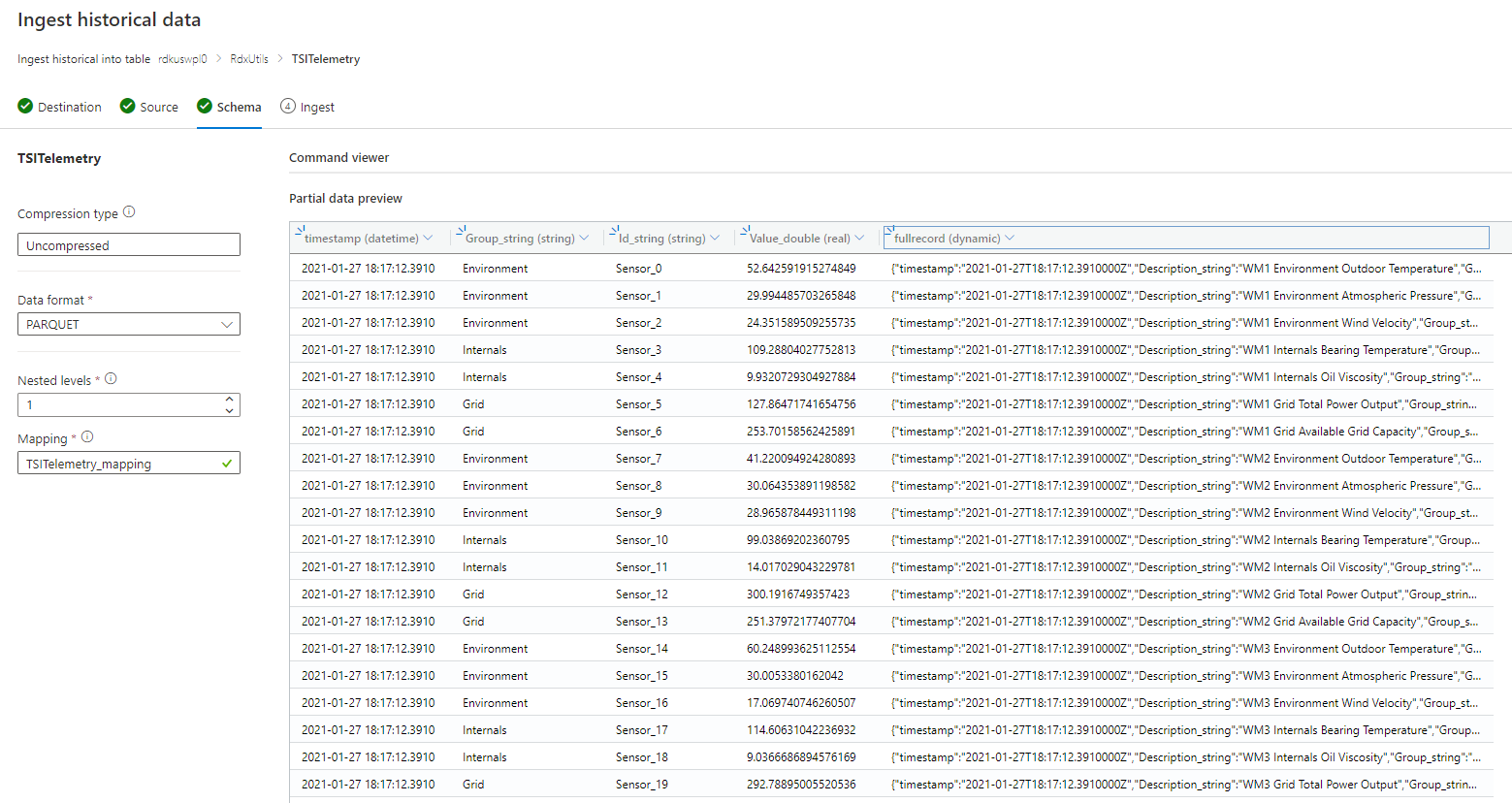
If schema is known or fixed
1. Confirm that the data looks correct. Correct any types if needed.
2. Select Next: Summary

Copy the LightIngest command and store it somewhere so you can use it in the next step.

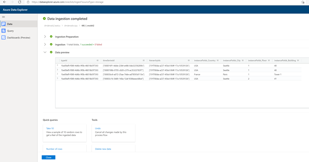
Data Ingestion

Before ingesting data you need to install the LightIngest tool. The command generated from One-Click tool includes a SAS token. It’s best to generate a new one so that you have control over the expiration time. In the portal, navigate to the Blob Container for the TSI Environment and select on ‘Shared access token’

Note

It’s also recommended to scale up your cluster before kicking off a large ingestion. For instance, D14 or D32 with 8+ instances.

Set the following
1. Permissions: Read and List
2. Expiry: Set to a period you’re comfortable that the migration of data will be complete
Select on ‘Generate SAS token and URL’ and copy the ‘Blob SAS URL’
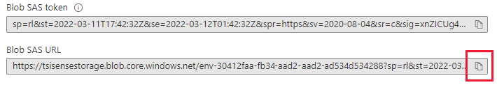
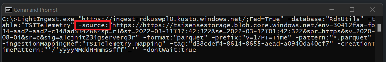
Go to the LightIngest command that you copied previously. Replace the -source parameter in the command with this ‘SAS Blob URL’
Option 1: Ingest All Data. For smaller environments, you can ingest all of the data with a single command.
1. Open a command prompt and change to the directory where the LightIngest tool was extracted to. Once there, paste the LightIngest command and execute it.
Option 2: Ingest Data by Year or Month. For larger environments or to test on a smaller data set you can filter the Lightingest command further.
1. By Year: Change your -prefix parameter
  - Before: -prefix:"V=1/PT=Time"
  - After: -prefix:"V=1/PT=Time/Y=<Year>"
  - Example: -prefix:"V=1/PT=Time/Y=2021"
2. By Month: Change your -prefix parameter
  - Before: -prefix:"V=1/PT=Time"
  - After: -prefix:"V=1/PT=Time/Y=<Year>/M=<month #>"
  - Example: -prefix:"V=1/PT=Time/Y=2021/M=03"

Once you’ve modified the command, execute it like above. One the ingestion is complete (using monitoring option below) modify the command for the next year and month you want to ingest.

Monitoring Ingestion

The LightIngest command included the -dontWait flag so the command itself won’t wait for ingestion to complete. The best way to monitor the progress while it’s happening is to utilize the “Insights” tab within the portal. Open the Azure Data Explorer cluster’s section within the portal and go to ‘Monitoring | Insights’

You can use the ‘Ingestion (preview)’ section with the below settings to monitor the ingestion as it’s happening

Time range: Last 30 minutes
Look at Successful and by Table
If you have any failures, look at Failed and by Table

You’ll know that the ingestion is complete once you see the metrics go to 0 for your table. If you want to see more details, you can use Log Analytics. On the Azure Data Explorer cluster section select on the ‘Log’ tab:

Useful Queries

Understand Schema if Dynamic Schema is used

| project p=treepath(fullrecord)
| mv-expand p 
| summarize by tostring(p)

Accessing values in array

| where id_string == "a"
| summarize avg(todouble(fullrecord.['nestedArray_v_double'])) by bin(timestamp, 1s)  
| render timechart

Migrating Time Series Model (TSM) to Azure Data Explorer

The model can be download in JSON format from TSI Environment using TSI Explorer UX or TSM Batch API. Then the model can be imported to another system like Azure Data Explorer.

Download TSM from TSI UX.
Delete first three lines using VSCode or another editor.
Using VSCode or another editor, search and replace as regex \},\n \{ with }{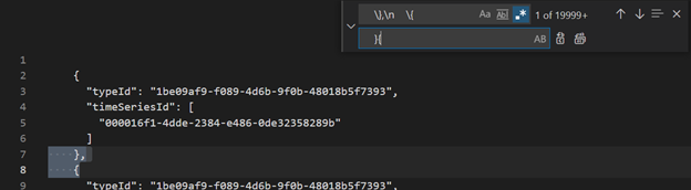
Ingest as JSON into ADX as a separate table using Upload from file functionality.

Translate Time Series Queries (TSQ) to KQL

GetEvents

{
  "getEvents": {
    "timeSeriesId": [
      "assest1",
      "siteId1",
      "dataId1"
    ],
    "searchSpan": {
      "from": "2021-11-01T00:00:0.0000000Z",
      "to": "2021-11-05T00:00:00.000000Z"
    },
    "inlineVariables": {},
  }
}

events
| where timestamp >= datetime(2021-11-01T00:00:0.0000000Z) and timestamp < datetime(2021-11-05T00:00:00.000000Z)
| where assetId_string == "assest1" and siteId_string == "siteId1" and dataid_string == "dataId1"
| take 10000

GetEvents with filter

{
  "getEvents": {
    "timeSeriesId": [
      "deviceId1",
      "siteId1",
      "dataId1"
    ],
    "searchSpan": {
      "from": "2021-11-01T00:00:0.0000000Z",
      "to": "2021-11-05T00:00:00.000000Z"
    },
    "filter": {
      "tsx": "$event.sensors.sensor.String = 'status' AND $event.sensors.unit.String = 'ONLINE"
    }
  }
}

events
| where timestamp >= datetime(2021-11-01T00:00:0.0000000Z) and timestamp < datetime(2021-11-05T00:00:00.000000Z)
| where deviceId_string== "deviceId1" and siteId_string == "siteId1" and dataId_string == "dataId1"
| where ['sensors.sensor_string'] == "status" and ['sensors.unit_string'] == "ONLINE"
| take 10000

GetEvents with projected variable

{
  "getEvents": {
    "timeSeriesId": [
      "deviceId1",
      "siteId1",
      "dataId1"
    ],
    "searchSpan": {
      "from": "2021-11-01T00:00:0.0000000Z",
      "to": "2021-11-05T00:00:00.000000Z"
    },
    "inlineVariables": {},
    "projectedVariables": [],
    "projectedProperties": [
      {
        "name": "sensors.value",
        "type": "String"
      },
      {
        "name": "sensors.value",
        "type": "bool"
      },
      {
        "name": "sensors.value",
        "type": "Double"
      }
    ]
  }
}

events
| where timestamp >= datetime(2021-11-01T00:00:0.0000000Z) and timestamp < datetime(2021-11-05T00:00:00.000000Z)
| where deviceId_string== "deviceId1" and siteId_string == "siteId1" and dataId_string == "dataId1"
| take 10000
| project timestamp, sensorStringValue= ['sensors.value_string'], sensorBoolValue= ['sensors.value_bool'], sensorDoublelValue= ['sensors.value_double']

AggregateSeries

{
  "aggregateSeries": {
    "timeSeriesId": [
      "deviceId1"
    ],
    "searchSpan": {
      "from": "2021-11-01T00:00:00.0000000Z",
      "to": "2021-11-05T00:00:00.0000000Z"
    },
    "interval": "PT1M",
    "inlineVariables": {
      "sensor": {
        "kind": "numeric",
        "value": {
          "tsx": "coalesce($event.sensors.value.Double, todouble($event.sensors.value.Long))"
        },
        "aggregation": {
          "tsx": "avg($value)"
        }
      }
    },
    "projectedVariables": [
      "sensor"
    ]
  }

events
| where timestamp >= datetime(2021-11-01T00:00:00.0000000Z) and timestamp < datetime(2021-11-05T00:00:00.0000000Z)
| where  deviceId_string == "deviceId1"
| summarize avgSensorValue= avg(coalesce(['sensors.value_double'], todouble(['sensors.value_long']))) by bin(IntervalTs = timestamp, 1m)
| project IntervalTs, avgSensorValue

AggregateSeries with filter

{
  "aggregateSeries": {
    "timeSeriesId": [
      "deviceId1"
    ],
    "searchSpan": {
      "from": "2021-11-01T00:00:00.0000000Z",
      "to": "2021-11-05T00:00:00.0000000Z"
    },
    "filter": {
      "tsx": "$event.sensors.sensor.String = 'heater' AND $event.sensors.location.String = 'floor1room12'"
    },
    "interval": "PT1M",
    "inlineVariables": {
      "sensor": {
        "kind": "numeric",
        "value": {
          "tsx": "coalesce($event.sensors.value.Double, todouble($event.sensors.value.Long))"
        },
        "aggregation": {
          "tsx": "avg($value)"
        }
      }
    },
    "projectedVariables": [
      "sensor"
    ]
  }
}

events
| where timestamp >= datetime(2021-11-01T00:00:00.0000000Z) and timestamp < datetime(2021-11-05T00:00:00.0000000Z)
| where  deviceId_string == "deviceId1"
| where ['sensors.sensor_string'] == "heater" and ['sensors.location_string'] == "floor1room12"
| summarize avgSensorValue= avg(coalesce(['sensors.value_double'], todouble(['sensors.value_long']))) by bin(IntervalTs = timestamp, 1m)
| project IntervalTs, avgSensorValue

Migration from TSI Power BI Connector to ADX Power BI Connector

The manual steps involved in this migration are

Convert Power BI query to TSQ
Convert TSQ to KQL Power BI query to TSQ: The Power BI query copied from TSI UX Explorer looks like as shown below

For Raw Data(GetEvents API)

{"storeType":"ColdStore","isSearchSpanRelative":false,"clientDataType":"RDX_20200713_Q","environmentFqdn":"6988946f-2b5c-4f84-9921-530501fbab45.env.timeseries.azure.com", "queries":[{"getEvents":{"searchSpan":{"from":"2019-10-31T23:59:39.590Z","to":"2019-11-01T05:22:18.926Z"},"timeSeriesId":["Arctic Ocean",null],"take":250000}}]}

To convert it to TSQ, build a JSON from the above payload. The GetEvents API documentation also has examples to understand it better. Query - Execute - REST API (Azure Time Series Insights) | Microsoft Docs
The converted TSQ looks like as shown below. It's the JSON payload inside “queries”

{
  "getEvents": {
    "timeSeriesId": [
      "Arctic Ocean",
      "null"
    ],
    "searchSpan": {
      "from": "2019-10-31T23:59:39.590Z",
      "to": "2019-11-01T05:22:18.926Z"
    },
    "take": 250000
  }
}

For Aggradate Data(Aggregate Series API)

For single inline variable, PowerBI query from TSI UX Explorer looks like as shown bellow:

{"storeType":"ColdStore","isSearchSpanRelative":false,"clientDataType":"RDX_20200713_Q","environmentFqdn":"6988946f-2b5c-4f84-9921-530501fbab45.env.timeseries.azure.com", "queries":[{"aggregateSeries":{"searchSpan":{"from":"2019-10-31T23:59:39.590Z","to":"2019-11-01T05:22:18.926Z"},"timeSeriesId":["Arctic Ocean",null],"interval":"PT1M", 		"inlineVariables":{"EventCount":{"kind":"aggregate","aggregation":{"tsx":"count()"}}},"projectedVariables":["EventCount"]}}]}

To convert it to TSQ, build a JSON from the above payload. The AggregateSeries API documentation also has examples to understand it better. Query - Execute - REST API (Azure Time Series Insights) | Microsoft Docs
The converted TSQ looks like as shown below. It's the JSON payload inside “queries”

{
  "aggregateSeries": {
    "timeSeriesId": [
      "Arctic Ocean",
      "null"
    ],
    "searchSpan": {
      "from": "2019-10-31T23:59:39.590Z",
      "to": "2019-11-01T05:22:18.926Z"
    },
    "interval": "PT1M",
    "inlineVariables": {
      "EventCount": {
        "kind": "aggregate",
        "aggregation": {
          "tsx": "count()"
        }
      }
    },
    "projectedVariables": [
      "EventCount",
    ]
  }
}

For more than one inline variable, append the json into “inlineVariables” as shown in the example below. The Power BI query for more than one inline variable looks like:

{"storeType":"ColdStore","isSearchSpanRelative":false,"clientDataType":"RDX_20200713_Q","environmentFqdn":"6988946f-2b5c-4f84-9921-530501fbab45.env.timeseries.azure.com","queries":[{"aggregateSeries":{"searchSpan":{"from":"2019-10-31T23:59:39.590Z","to":"2019-11-01T05:22:18.926Z"},"timeSeriesId":["Arctic Ocean",null],"interval":"PT1M", "inlineVariables":{"EventCount":{"kind":"aggregate","aggregation":{"tsx":"count()"}}},"projectedVariables":["EventCount"]}}, {"aggregateSeries":{"searchSpan":{"from":"2019-10-31T23:59:39.590Z","to":"2019-11-01T05:22:18.926Z"},"timeSeriesId":["Arctic Ocean",null],"interval":"PT1M", "inlineVariables":{"Magnitude":{"kind":"numeric","value":{"tsx":"$event['mag'].Double"},"aggregation":{"tsx":"max($value)"}}},"projectedVariables":["Magnitude"]}}]}

{
  "aggregateSeries": {
    "timeSeriesId": [
      "Arctic Ocean",
      "null"
    ],
    "searchSpan": {
      "from": "2019-10-31T23:59:39.590Z",
      "to": "2019-11-01T05:22:18.926Z"
    },
    "interval": "PT1M",
    "inlineVariables": {
      "EventCount": {
        "kind": "aggregate",
        "aggregation": {
          "tsx": "count()"
        }
      },
      "Magnitude": {
        "kind": "numeric",
        "value": {
          "tsx": "$event['mag'].Double"
        },
        "aggregation": {
          "tsx": "max($value)"
        }
      }
    },
    "projectedVariables": [
      "EventCount",
      "Magnitude",
    ]
  }
}

If you want to query the latest data("isSearchSpanRelative": true), manually calculate the searchSpan as mentioned below
- Find the difference between “from” and “to” from the Power BI payload. Let’s call that difference as “D” where “D” = “from” - “to”
- Take the current timestamp(“T”) and subtract the difference obtained in first step. It will be new “from”(F) of searchSpan where “F” = “T” - “D”
- Now, the new “from” is “F” obtained in step 2 and new “to” is “T”(current timestamp)