How to filter table that uses a formula to filter tables in Excel?

Question

Hello everyone,

I have a file, that has two sheets. The following image is for Sheet1 it has three tables:

And in Sheet2, I have table that has a formula to filter the three tables that exist in Sheet1. So please see the following image it's for Sheet2, and the formula used to filter that tables is this:

= IFERROR(

VSTACK(

FILTER(Sheet1!A3:E7, Sheet1!B3:B7 = F1,"Empty or Error"),

FILTER(Sheet1!G3:K7, Sheet1!H3:H7 = F1,"Empty or Error"),

FILTER(Sheet1!M3:Q7, Sheet1!N3:N7 = F1, "Empty or Error")

), "Empty or Error")

This formula is located in cell F3 in Sheet2, and the following image is for Sheet2

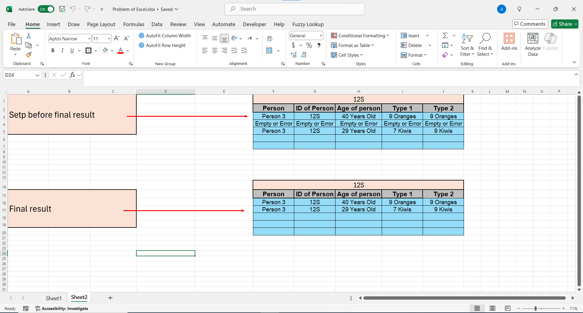
The problem comes when I delete a cell from any table in Sheet1 so in this example If I delete the content of cell H5 in Sheet1 I get unwanted row in the table that contains "Empty or Error" so I'm forced to use other table and other formula to filter that table to remove that row from the result, I know I can make that row empty instead of having "Empty or Error" but I don't want empty rows I want only rows that contain text. Note that, cell H5 in Sheet1 contains "12S" and when I delete its content I get the following result as it illustrated in the following image:

In the step before the final result, the formula used in the table is the same formula that I gave above, and now in the second table which contains the final result I have the following formula and it's located in cell F16:

=FILTER(F3:J5, NOT(BYROW(F3:J5, LAMBDA(row, ISNUMBER(MATCH("Empty or Error", row, 0))))))

In this case I want to combine these two steps so to remove first table and directly get the final result without depending in the first table. How to do that?

You can download and see the file by the following link from OneDrive:
https://1drv.ms/x/c/3b862aaec36e5e46/EYahg-18xBhFkYmb8ERp6R4B881RK_WrL3DNayI5tSg5vA?e=bNkXlk

Extra information:
I have license for Microsoft 365. Also, I have license for Microsoft Office Home and Business 2024.

Answer 1

For example:

=IFERROR(LET(
    combined, VSTACK(
        FILTER(Sheet1!A3:E7, Sheet1!B3:B7 = F1, ""),
        FILTER(Sheet1!G3:K7, Sheet1!H3:H7 = F1, ""),
        FILTER(Sheet1!M3:Q7, Sheet1!N3:N7 = F1, "")
        ),
    FILTER(combined, TAKE(combined, , 1)<>"")),
    "Empty or Error")

Answer 2

Hi,

Try this formula to cell F3 of Sheet2:

=LET(vs, VSTACK(Sheet1!A3:E7, Sheet1!G3:K7, Sheet1!M3:Q7), FILTER(vs, CHOOSECOLS(vs, 2) = F1))

Hope this helps.