Create an Excel Services dashboard using an OData data feed

Article
04/27/2023

APPLIES TO: yes-img-13 2013 no-img-16 2016 no-img-19 2019 no-img-se Subscription Edition no-img-sop SharePoint in Microsoft 365

This article describes, step by step, how to use Excel 2016 to create a basic dashboard that contains two reports and two filters. The example dashboard described in this article resembles the following image:

Figure: Basic Excel Services dashboard that contains two reports and two slicers

Basic Excel Services dashboard

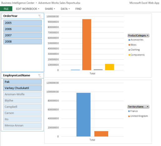
Our example dashboard uses data that is imported into Excel using an OData data feed. This makes it possible to publish the workbook to a library in SharePoint Server 2013. By following the steps in this article, you'll learn how to import data into Excel, use that data to create reports in a worksheet, and connect filters to those reports.

Before you begin

Before you begin this operation, review the following information about prerequisites:

Excel 2016 must be installed on the computer that you are using to create and publish the dashboard.
This scenario uses Adventure Works sample data and a Business Intelligence Center site in SharePoint Server 2013.

The Adventure Works sample data that we'll use is available via an OData data feed. For more information, see AdventureWorks OData Feed (on CodePlex).

If you do not have a Business Intelligence Center site, have an IT administrator configure it for you by using the instructions in Configure AdventureWorks for Business Intelligence solutions.
Excel Services must be configured to support Data Models. For information about how to deploy Excel Services, see Configure Excel Services in SharePoint Server 2013 and Manage Excel Services data model settings (SharePoint Server 2013).

Plan the dashboard

Before you begin to create a dashboard, we recommend that you create a dashboard plan. The plan does not have to be extensive or complex. However, it should give you an idea of what you want to include in the dashboard. To help you prepare a dashboard plan, consider questions such as the following:

Who will use the dashboard?
What kinds of information do they want to see?
Does data exist that you can use to create the dashboard?

Our example dashboard is designed to be a prototype that you can use to learn how to create and publish Excel Services dashboards. To show how we might create a dashboard plan for a similar dashboard, see the following table.

Table: Basic plan for our example dashboard

Question	Response
Who will use the dashboard?	The dashboard is intended for use by sales representatives, sales managers, corporate executives, and other stakeholders who are interested in sales information for the fictitious company Adventure Works Cycles.
How will the dashboard be used? That is, what kinds of information do the dashboard consumers want to see?	Sales representatives, managers, executives, and other dashboard consumers want to use the dashboard to view, explore, and analyze data. At a minimum, the dashboard consumers want to see the following kinds of information: Sales amounts across different geographical areas Sales amounts across different geographical areas Sales amounts for different years Sales amounts for different sales representatives Dashboard consumers want to use the dashboard to view, explore, and analyze data to obtain answers to specific questions. The dashboard consumers also want to be able to use filters to focus on more specific information, such as sales for a particular year or a particular sales representative.
Does data exist that we can use to create the dashboard?	Yes. The Adventure Works sample database that we'll use contains the data that we can use for the dashboard.
What items should the dashboard contain?	Our example dashboard includes the following items: Data that is imported by using an OData data feed A chart showing product sales information for different geographical areas A chart showing sales information for different geographical areas A slicer that dashboard consumers can use to view information for a particular year A slicer that dashboard consumers can use to view information for a particular sales representative
Where will the dashboard be published?	Because our example dashboard uses native data in Excel, the dashboard can be published to a SharePoint library in SharePoint Server 2013 or in SharePoint in Microsoft 365. This enables people to consume the dashboard content internally or via an Internet connection. It also enables people to view the dashboard by using a mobile device, such as Apple iPad or Windows 8 tablet.

Now that we have created our dashboard plan, we can begin to create the dashboard.

Create the dashboard

To create the dashboard, we begin by creating a data connection. Then, we use that data connection to import data into Excel. Next, we create the reports and the filter that we want to use. After that, we publish the workbook to SharePoint Server 2013.

Part 1: Get data into Excel

Our example dashboard uses data that is imported into Excel via an OData data feed to connect to Adventure Works sample data. For more information, see AdventureWorks OData Feed (on CodePlex). We begin by importing data into Excel.

To import data into Excel by using an OData data feed

Open Microsoft Excel.
Choose Blank workbook to create a workbook.
On the Data tab, choose Get External Data group, choose From Other Sources, and then choose From OData Data Feed.

The Data Connection Wizard opens.
On the Connect to Database Server page, in the Location of the data feed box, specify the website address (URL) for the data feed.

For our example dashboard, we used https://services.odata.org/AdventureWorksV3/AdventureWorks.svc.
In the Log on credentials section, take one of the following steps:

Choose Use the sign-in information for the person opening this file, and then choose the Next button.
Choose Use this name and password, specify an appropriate user name and password, and then choose the Next button.

Tip

If you don't know which option to choose, contact a SharePoint admin.

On the Select Tables page, choose the CompanySales table and the TerritorySalesDrilldown table. Then choose the Next button.
On the Save Data Connection File and Finish page, choose the Finish button.
On the Import Data page, take the following steps:
Select the Table option.
Make sure the Add this data to the Data Model option is selected.
Choose the OK button.

Sheet2 and Sheet3 that contain data are added to the workbook.
Keep Excel open.

At this point, we have imported data into Excel by using an OData data feed. The next step is to create a relationship between the tables of data. To do that, we'll use the Power Pivot Add-In for Excel. If the PowerPivot tab is not visible in Excel, enable the add-in by using the following procedure.

To enable the PowerPivot add-in for Excel

In Excel, on the File tab, choose Options.
In the Excel Options dialog, choose Add-Ins.
In the Manage list, choose COM Add-Ins, and then choose the Go button to open the COM Add-Ins dialog.
Select Microsoft Office PowerPivot for Excel 2013, and then choose OK. The PowerPivot tab is now visible in Excel.
Keep Excel open.

Now that the Power Pivot add-in for Excel is enabled, the next step is to create a relationship between the tables of data. This will enable us to create reports and filters using data from the two tables.

To create a relationship between tables in a Data Model

In Excel, on the PowerPivot tab, in the Data Model group, choose Manage. Power Pivot for Excel opens.
In the PowerPivot for Excel window, on the Design tab, in the Relationships group, choose Create Relationship.
In the Create Relationship dialog, specify the following settings:

In the Table list, verify that CompanySales is selected.
In the Column list, choose ID.
In the Related Lookup Table list, choose TerritorySalesDrilldown.
In the Related Column Lookup list, verify that ID is selected.

Then choose the Create button.

Close the PowerPivot for Excel window, but keep Excel open.

At this point, we have imported two tables of data into Excel. We have also created a relationship between the tables so that we can create reports and filters that use the two tables as a single data source.

Part 2: Create reports

For our example dashboard, we'll create two reports, as described in the following table:

Table: Dashboard reports

Report Type	Report Name	Description
PivotChart report	ProductSales	Bar chart that shows sales amounts across different product categories.
PivotChart report	GeoSales	Bar chart that shows sales amounts across different sales geographical areas.

We begin by creating the ProductSales report.

To create the ProductSalesReport chart

In Excel, select Sheet1.
On the Insert tab, in the Charts section, choose PivotChart.The Create PivotChart dialog appears.
In the Choose the data that you want to analyze section, choose the Use an external data source option, and then choose the Choose Connection button.

The Existing Connections dialog appears.
On the Tables tab, select the Tables in Workbook Data Model option, and then choose the Open button.
In the Create PivotChart dialog, choose the Existing Worksheet option, and then choose the OK button.

Chart1 opens for editing.
In the PivotChart Fields list, specify the following options:

From the CompanySales section, drag ProductCategory to the Legend (Series) field well.
In the CompanySales section, select the check box next to Sales.

The chart updates to display sales amounts across different product categories.

Move the PivotChart report closer to the upper-left corner of the worksheet. To do this, drag the report so that the upper-left corner aligns with the upper-left corner of cell D1 in the worksheet.
To avoid confusion about report names later, we'll specify a new name for the report. To do that, take the following steps:
Somewhere in the PivotChart report, right-click, and then choose PivotChart Options.
In the PivotChart Options dialog, in the PivotChart Name box, type ProductSalesReport.

Tip

Make sure that the name that you specify contains only alphanumeric characters (no spaces).
Choose the OK button.
Save the workbook by using a file name such as Adventure Works Sales Reports.
Keep the workbook open.

At this point, we have created a PivotChart report showing product sales. The next step is to create a PivotChart report that shows sales amounts across different geographical locations.

To create the GeoSalesReport chart

In Excel, on the same worksheet that was used to create the ProductSales report, choose cell B17.
On the Insert tab, choose PivotChart.
In the Choose the data that you want to analyze section, choose the Use an external data source option, and then choose the Choose Connection button.

The Existing Connections dialog appears.
On the Tables tab, select the Tables in Workbook Data Model option, and then choose the Open button.
In the Create PivotChart dialog, choose the Existing Worksheet option, and then choose the OK button.

PivotChart2 opens for editing.
In the PivotChart Fields list, specify the following options:

In the CompanySales section, select Sales.
In the TerritorySalesDrilldown section, drag TerritoryName to the Legend (Series) field well.

The report updates to display a chart showing sales amounts for different geographical areas.

Move the report so that its upper-left corner aligns with the upper-left corner of cell D16.
To specify a name for the report, take the following steps:
Somewhere in the report, right-click and then choose PivotChart Options.
In the PivotChart Name box, type GeoSalesReport.
Choose OK.
On the File tab, choose the Save button.
Keep the workbook open.

At this point, we have created our two reports for our basic dashboard. The next step is to create filters.

Part 3: Add filters

Using Excel, there are several different kinds of filters we can create and add to a dashboard. For example, we can create a simple filter by putting a field in the Filter section of the Fields list. We can create a slicer, or, if we are using a multidimensional data source such as Analysis Services, we can create a timeline control. For this example dashboard, we'll create two slicers. This filter will enable people to view information for a particular year or a particular sales representative.

To add slicers to the dashboard

In Excel, on the same worksheet that was used to create the reports, choose cell A1.
On the Insert tab, in the Filter group, choose Slicer.

The Existing Connections dialog appears.
On the Data Model tab, select the Tables in Workbook Data Model option, and then choose the Open button.
In the Insert Slicers dialog, take the following steps:
In the CompanySales section, choose OrderYear.
In the TerritorySalesDrilldown section, choose EmployeeLastName.
Choose the OK button.
Move the slicers so that the upper-left corner of the OrderYear slicer aligns with the upper-left corner of cell A1, and the EmployeeLastName slicer is positioned immediately below the OrderYear slicer.
Connect the slicers to the reports by following these steps:
Select the OrderYear slicer.
On the Options tab, in the Slicer group, choose the Report Connections toolbar command.
In the Report Connections dialog, choose the ProductSalesReport and GeoSalesReport check boxes, and then choose the OK button.
Repeat these steps for the EmployeeLastName slicer.
On the File tab, choose the Save button.
Keep the Excel workbook open.

At this point, we have created a dashboard. The next step is to publish it to SharePoint Server 2013, where it can be used by others.

Publish the dashboard

To publish the workbook to SharePoint Server 2013, we'll follow a two-step process. First, we make some adjustments that affect how the workbook is displayed. Then, we publish the workbook to a SharePoint library.

We begin by making adjustments to the workbook. By default, our example dashboard displays gridlines on the worksheet that contains our dashboard. In addition, by default, the worksheet is called Sheet1. We can make some minor adjustments that will improve how the dashboard will be displayed.

To make minor display improvements to the workbook

In Excel, choose the View tab.
To remove gridlines from the view, on the View tab, in the Show group, clear the Gridlines check box.
To remove row and column headings, on the View tab, in the Show group, clear the Headings check box.
To rename the worksheet, right-click its tab where it says Sheet1, and then choose Rename. Immediately type a new name for the worksheet, such as SalesInfo, and then press the Enter key.
On the File tab, choose Save.
Close Excel.

The next step is to publish the workbook to a SharePoint library. The workbook uses native data that we imported into Excel, which means that we can publish it to a library in SharePoint Server 2013. Use one of the following procedures to publish the workbook.

To publish the workbook to a library in SharePoint Server 2013

Open a web browser.
In the address line, type the SharePoint address to a library in SharePoint Server 2013.

For our example, we used the Documents library that is available by default in a Business Intelligence Center site. The SharePoint address we used resembles http://servername/sites/bicenter/documents.

Tip

Contact a SharePoint admin if you do not know the SharePoint address for a library that you can use.
In the Documents library, click + New Document to open the Add a Document dialog.
Choose Browse, and then use the Choose File to Upload dialog to select the Adventure Works Sales Reports workbook. Then choose Open.
In the Add a document dialog, choose OK. The workbook is added to the library.

Now that we have created and published the dashboard, we can use it to explore data.

Use the dashboard

After the dashboard was published to SharePoint Server 2013, it is available for people to view and use it.

To open the dashboard

Open a web browser.
In the address bar, type the address to the Business Intelligence Center site where the dashboard was published.
Choose Site Contents, and then choose Documents.
Choose the Adventure Works Sales Reports dashboard. The dashboard opens for viewing in a browser window.

Now that the dashboard is open for viewing, we can use it to obtain answers to specific questions, such as those that are described in the following table.

Table: Using the dashboard to obtain answers to specific questions

Question	Action
In 2005, which product category had the most sales?	In the OrderYear slicer, choose 2005. Notice that in the ProductSalesReport chart, the Bikes product category has the highest sales amount.
Which year had the highest amount of sales for the Bikes product category?	To find the answer, we'll use the Quick Explore feature. Follow these steps: Clear the OrderYear slicer. In the ProductSalesReport chart, select the Bikes bar. The Quick Explore button appears. Click (or tap) the Quick Explore button to open the Explore dialog. Expand CompanySales, choose OrderYear, and then choose Drill To OrderYear. The ProductSalesReport chart updates to show sales amounts for the Bikes product category. According to the ProductSalesReport chart, 2007 was the year in which this company had the highest sales amounts for the Bikes category.
In France, which product subcategory has the highest amount of sales?	To find the answer, we'll use the Quick Explore feature. Follow these steps: Refresh the browser window to restore the dashboard to its default view. In the GeoSalesReport chart, select the France bar to display the Quick Explore button. Click (or tap) the Quick Explore button. Expand CompanySales, choose ProductSubCategory, and then choose Drill To ProductSubCategory. The chart updates to display lots of products. Point to the tallest bar. A callout appears that indicates that bar corresponds to the Road Bikes subcategory. According to the GeoSalesReport chart, Road Bikes has the highest amount of sales in France for this company.