Excel Conditional Formatting

Question

I’m wanting to make cells turn green, yellow, or red based on days out from the current =now() date and was wondering what the formulas for those would be. I’m wanting the days that are fine green, 6-8 months out to be yellow and expired to be red. I’m currently having trouble wording it.

Answer 1

Hi @William Deaver

1) Select the range you want to apply formatting to > Press Conditional Formatting > New Rule

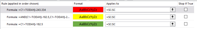
2) Add the following rules (You will need to change C1 to what column you actually utilizing for the range -- I used column C in my example):

I used the calculation, 6 months = 182.5 days AND 8 months = 243.334 days.

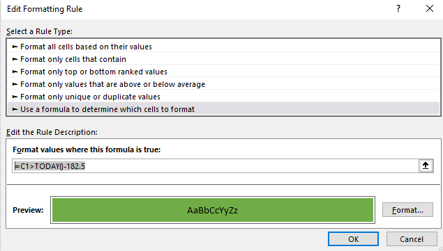
a) Add for up to 6 months:

=C1>TODAY()-182.5

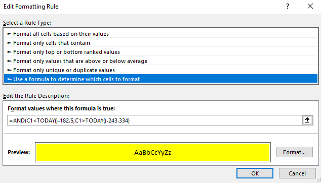
b) Add for 6-8 months range:

=AND(C1<TODAY()-182.5,C1>TODAY()-243.334)

c) Add for more than 8 months:

=C1<TODAY()-243.334

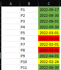
3) Hit Apply and you should see the following (I applied to column C)

---

If this is helpful please accept answer.

Answer 2

Hi @William Deaver

Welcome to Q&A forum ~

> I’m wanting the days that are fine green, 6-8 months out to be yellow and expired to be red. I’m currently having trouble wording it.

Actually, I am a little confused about your requests.

But to compare dates, as DillonJS suggested, you can use Today function, or you can use EDATE function.

If the your request is logically as follows：

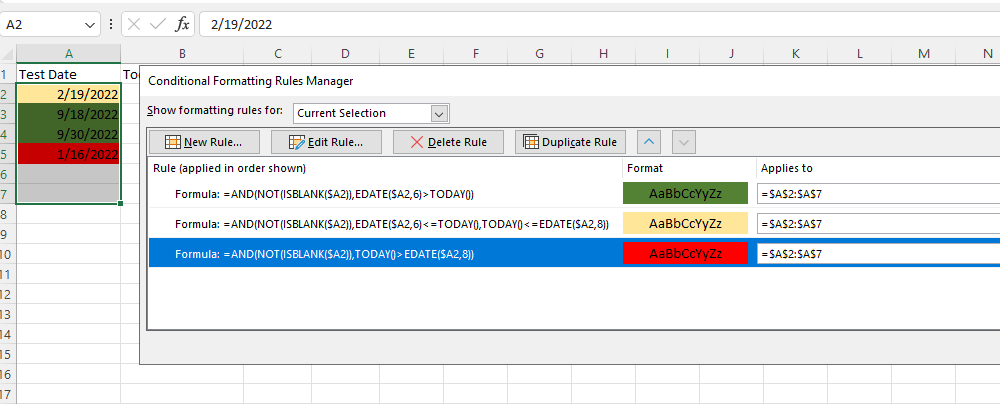
Green --- Dates + 6 months > Today ()
Yellow --- Dates + 6 months <= Today () <= Dates +8 months
Red --- Dates +8 months < Today

Then you can try following conditional formulas:

Green --- =AND(NOT(ISBLANK($A2)),EDATE($A2,6)>TODAY())
Yellow --- =AND(NOT(ISBLANK($A2)),EDATE($A2,6)<=TODAY(),TODAY()<=EDATE($A2,8))
Red --- =AND(NOT(ISBLANK($A2)),TODAY()>EDATE($A2,8))

Any updates, welcome to post back.

---

If the answer is helpful, please click "Accept Answer" and kindly upvote it. If you have extra questions about this answer, please click "Comment".
Note: Please follow the steps in our documentation to enable e-mail notifications if you want to receive the related email notification for this thread.

---