Power query M pivot table/filter function

Question

Hi, I have a problem that I can solve.
I have a database with sales data. I want to be able to show this data as sales per product group in an Excel pivot table,
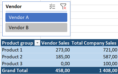
1 column with the total sales of the company for each product group and 1 column with only the sales from one or more specifc vendor/s that I specify with a filter in the Excel pivot table.

I dont know how to keep the total sales of the product group when I use the filter for a specific vendor?

I know I can make a specific column in my power query editor but then I have to specify what vendor it should be already there and I need to be able to choose this with the filter in the Excel Pivot table.

I would like it to look similar to this (i don't know if I managed to upload the image.

Answer 1

Hi @Fredrik Söderholm Pettersson

A picture of your source table would have helped... Assuming Table1 loaded as is to the Data Model:

1/ Create measure Total Sales: =SUM(Table1[Amount])
With your scenario use it for your expected Vendor Sales column

2/ Create measure Total Company Sales: =CALCULATE([Total Sales];ALL(Table1[Vendor]))

Corresponding sample available here