Excel Formula to find Unique values from Data Table

Question

Thank you for taking the time to read my question.

I have a data table with many customers. Each customer has many sites. I'm wondering if it's possible to use Excel formulas to return the unique list of sites based on the Customer name entered into a cell. Next I'd like to be able to show the unique values horizontally.

Is this possible or do I need to write a quick macro?

Data Table:

Customer 1 Site 1 Other data
Customer 1 Site 1 Other data
Customer 1 Site 1 Other data
Customer 1 Site 1 Other data
Customer 1 Site 1 Other data
Customer 1 Site 2 Other data
Customer 1 Site 2 Other data
Customer 1 Site 2 Other data
Customer 1 Site 2 Other data
Customer 1 Site 3 Other data
Customer 2 Site A Other data
Customer 2 Site A Other data
Customer 2 Site B Other data
Customer 2 Site B Other data

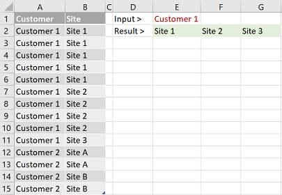
User Input: Customer 1

Result I'd like to see

    A           B         C

1| Site 1 | Site 2 | Site 3

I found the Unique() function but I need to pass it a range of cells and I'm not sure how to do that. I also found the Transpose() function which I thought I could put the Unique() function in.

=Transpose(Unique("The range I'm not sure how to pass",True,True))

Thanks

Answer 1

@b bb ,
Welcome to Q&A forum!

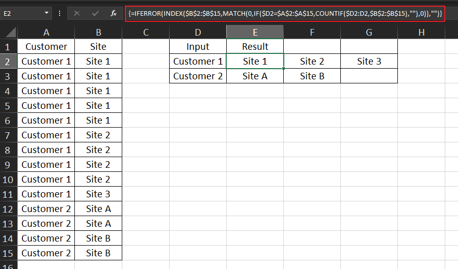
Please check whether the following formula is helpful to you, since it is an array formula, please press Ctrl+Shift+Enter to check after typing.
For more information about INDEX: INDEX function.

=IFERROR(INDEX($B$2:$B$15,MATCH(0,IF($D2=$A$2:$A$15,COUNTIF($D2:D2,$B$2:$B$15),""),0)),"")  

Any updates, please let me know.

---

If an Answer is helpful, please click "Accept Answer" and upvote it.
Note: Please follow the steps in our documentation to enable e-mail notifications if you want to receive the related email notification for this thread.

Answer 2

Hi,

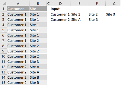
In cell D2, enter this formula

=UNIQUE(A2:A15)

In cell E2, enter this formula

=IFERROR(DROP(REDUCE("",D2#,LAMBDA(a,b,VSTACK(a,TOROW(UNIQUE(FILTER(B2:B15,A2:A15=b)))))),1),"")

Hope this helps.

Answer 3

Hi,

This Power Query code works as well

let
    Source = Excel.CurrentWorkbook(){[Name="Data"]}[Content],
    #"Removed Duplicates" = Table.Distinct(Source),
    #"Grouped Rows" = Table.Group(#"Removed Duplicates", {"Customer"}, {{"Count", each Table.AddIndexColumn(_,"Index",1)}}),
    #"Expanded Count" = Table.ExpandTableColumn(#"Grouped Rows", "Count", {"Site", "Index"}, {"Site", "Index"}),
    #"Added Prefix" = Table.TransformColumns(#"Expanded Count", {{"Index", each "Col " & Text.From(_, "en-IN"), type text}}),
    #"Pivoted Column" = Table.Pivot(#"Added Prefix", List.Distinct(#"Added Prefix"[Index]), "Index", "Site")
in
    #"Pivoted Column"