HELP ME WITH EXCEL FORMULA FOR MOVING DATA??

Question

I need to know what the VLOOKUP FORMULA is for moving numbers between these 2 sheets because I can not figure out the formula myself. I have tried all day, and I can not get it.

JUST LIKE IT SHOWS IN THE SCREENSHOT ABOVE. I have 2 sheets named "Testing Day 1" and "Month 1 Week 1". I want to pull the number in cell Q12 from "Testing Day 1" and then drop that number into the cell B97 in "Month 1 Week 1".

I know I need to enter a VLOOKUP FORMULA (or another formula that does the same thing) into the cell B97 in Month 1 Week 1. But I don't know exactly how to enter all the variables in the formula to make it work. I do know the formula needs to look something like this though.

=VLOOKUP(Q12, Testing Day 1!$B$97, 14, FALSE)

I want to do the exact same thing in the screenshot below too. Pull the number from cell Q12 in Testing Day 1 and drop that number into cell C11 in Master File using a VLOOKUP FORMULA again (or another formula that does the same thing).

JUST PLEASE TELL ME HOW TO ENTER THIS FORMULA PROPERLY?? IT IS DRIVING ME COMPLETELY INSANE??

Answer 1

Try the following formulas. Note that the Table_Array must be in absolute format (with the $ signs)

The value to be found must be in the first column of the Table_Array and the returned value is from the column number counted from the first column of the Table_Array.

Sheet MONTH 1 (WEEK 1) cell B97

=VLOOKUP(A97,'TEST DAY 1'!$P$12:$Q$14,2,FALSE)

Sheet MASTER FILE SHEET cell C11

=VLOOKUP(A11,'TEST DAY 1'!$A$12:$Q$14,17,FALSE)

More information on Vlookup at the following link

https://support.microsoft.com/en-us/office/vlookup-function-0bbc8083-26fe-4963-8ab8-93a18ad188a1

Answer 2

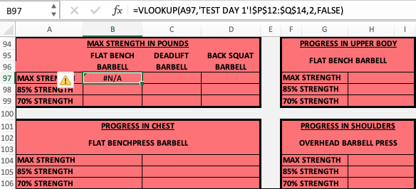
I'm confused by your first formula which is =VLOOKUP(A97,'TEST DAY 1' !$P$12:$Q$14,2,FALSE)

Because A97 and P12 are nothing. The cells A97 and P12 are just cells with the word "BENCH" in it. Why would two cells with a word in it, be included in the formula? I am not sure I understand that?

Everything else in your formula seems to make sense though. The formula is pulling data from the sheet "TEST DAY 1" so that is correct. The cell that the data is being pulled from is Q12 in the TEST DAY 1 sheet so that also makes sense. The number 2 represents column B because the data is being inserted into cell B97 in the sheet MONTH 1 WEEK 1 so that also makes sense. And the False makes sense too.

Unfortunately, both of your Formulas did not work. It gives me an error that says "Value Not Available Error". I have spoken to a few Excel Experts and NONE OF THEM have been able to get this formula to work in my worksheet. So I am really starting to think it can not be done.

I don't know what else to do.

As you can see in the screenshot. I entered your Formula into cell B97 and it did not work. Any idea why it won't work no matter what I do?

Once again, you can see in the screenshot below that the other formula did not work too. I put it into cell C11 but it does not work. Any idea why it won't work no matter what I do?

Any idea why it won't work no matter what I do?

Answer 3

Maybe I have not got the correct association with the sheet names.

If you can upload your workbook to OneDrive then I will try to assist further. Note that many business OneDrives do not permit sharing so doesn't work but otherwise should be OK. I have had some people who take a copy home and upload from their private Onedrive.

If the workbook contains sensitive data then make a copy and replace the sensitive data with dummy data.

Guidelines to upload a workbook on OneDrive. (If you already use OneDrive and your process for saving to it is different then you can probably start at step 8 to get the link but please zip the file before uploading.)

1. Zip your workbooks. Do not just save an unzipped workbook to OneDrive because the workbooks open with On-Line Excel and the limited functionality with the On-Line version causes problems.
2. To Zip a file: In Windows Explorer Right click on the selected file and select Send to -> Compressed (zipped) folder). By holding the Ctrl key and left click once on each file, you can select multiple workbooks before right clicking over one of the selections to send to a compressed file and they will all be included into the one Zip file.
3. Do not use 3rd party compression applications because I cannot unzip them. I do not clog up my computer with 3rd party apps when there are perfectly good apps supplied with windows.
4. Go to this link.  https://onedrive.live.com
5. Use the same login Id and Password that you use for this forum.
6. Select Upload under the blue bar across the top and browse to the zipped folder to be uploaded.
7. Select Open (or just double click). (Be patient and give it time to display the file after initially seeing the popup indicating it is done.)
8. Right click the file name in OneDrive.
9. Select Share.
10. Click the link icon (Looks like chain links) at the bottom left of the dialog (Just above "Copy link").
11. Click Copy button.
12. Change back to this forum and click the "Insert Hyperlink" icon at top of the posting editor (Icon looks like chain links).
13. Right click in the Web address field and right click and paste (or just Ctrl V to paste).
14. Click "Insert" Button.

Answer 4

I got it to work. A Microsoft Rep figured out the correct formula. This was the correct formula.

=VLOOKUP('TEST DAY 1'! A12,'TEST DAY 1'!A12:N14,13,FALSE)

Do you know if it's supposed to combine a VLOOKUP FORMULA with an IF STATEMENT or ISBLANK STATEMENT?? Because I want the formula to stay in the cell even if the data in the cell is deleted. Right now, if I delete the numbers in the cell, the formula in that cell gets deleted as well. But I want the formula to stay in that cell forever, even if the cell is empty or the numbers in the cell get deleted. Is it possible to combine the VLOOKUP FORMULA like the one above, with an IF STATEMENT or ISBLANK STATEMENT so the formula will always stay in the cell??

HERE IS THE LINK TO THE EXCEL WORKBOOK IF YOU WANT TO EXPERIMENT AND TEST OUT FORMULAS IN IT ANYWAY. I zipped the file as requested and followed your instructions by uploading it to OneDrive. Here is the link to it.

https://1drv.ms/u/s!AjCBMp0-Q-q0rVtQqOnQmkezOrSA?e=eOgj7j

SEE SCREENSHOT BELOW TO SEE THAT THE FORMULA FINALLY WORKED.

Answer 5

@AlexanderBouraad,

I have the file however, it is getting on towards beer o'clock for me so will probably be tomorrow before I do very much with it.