Can conditional formatting use RGB values specified in a set of cells?

Question

Let's say that I have three cells with RGB codes (one each for R, G, and B values). Is it possible to have a conditional format set up so that it will use the RGB values in those cells?

If, for example, I have the three cells as 255,0,0 (bright red), then cells that use that conditional format would show in bright red. If I decide to change the cells to bright blue (0,0,255), the conditional format would immediately recognize that change and apply it. So whenever I decide, for whatever reason, to use a different color, all I need do is change the RGB cell values and presto. In this way, a single conditional format would suffice, rather than a separate rule for each color I may want to use.

Answer 1

Hi Michael,

Thanks for posting in the forum.

From your post, I understand that you have three cells with text for example 1, 2 and 3 and the cells are filled with 255,0,0 (bright red) color and now you want to apply conditional value, if the value in the cell changes, the color changes to bright blue (0,0,255). Correct?

I have created a GIF for your reference.

If I misunderstood anything, please correct me and please provide us sample screenshot to understand your requirement better.

Thanks,

Neha

Answer 2

Hi Michael,

I've been wanting to do something just like that but gave up, so I hope someone provides the answer to your latest post!! I would use it right away.

Fingers crossed!

CB

Answer 3

Hello Neha,

Thanks for your reply and the GIF. However, this isn't what I'm asking for.

I understand the conditional formatting process, and what you have done. However, what I would like to do is avoid setting up multiple conditional rules in favor of using just one that would set the colors based on chosen values. Please see my uploaded image.

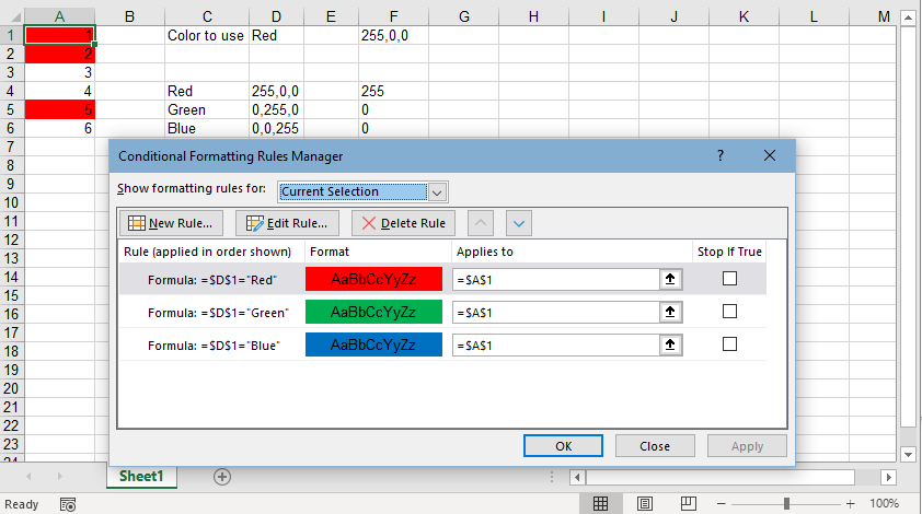
Here, I have a set of data in A1:A6, and I want to shade three cells with a color of my choosing. Currently, that is Red.

Cells C4:D6 is a color list, with color names and their RGB values. This list could be of any length, only depending on how many colors I'd like to use.

Cell D1 is a validated (by list) cell that refers to those color names in C4:D6 and returns the RGB values to cell F1. Cells F4, F5, and F6 hold the individual R, G, and B values from F1.

You can see the conditional formatting that I've used, which I have applied to cells A1, A2 and A5. Using this, when I select one of the colors in D1, those three cells will change to the appropriate color. This all works fine, and I've done that all over my various spreadsheets. But setting up these formats requires that I add another Rule to the conditional formatting for each color that I might want to use. For example, if I wanted to also use Orange, Yellow and Purple, I would have to add three more rules to this conditional format. And each Rule requires that I go into the Format and hand-select the appropriate color from the charts, just as you have done in your example.

So, let's say for my purposes that I want to use 12 colors. I would have 12 Rules in this conditional format, and would need to hand-pick the colors for each line. This works, but is very tedious.

What I would like is to define a set of colors, and then have conditional formatting refer to the RGB values in cell F1 (or possibly the three cells F4:F6, if it's necessary to pass the individual values).

My aim is to say "Hey, Excel, shade the cells I've indicated to the color that I've chosen in cell D1." In this way, a single Rule could accommodate any number of colors of my choosing, rather than having to define an individual rule for each color (and that requires me to manually choose the color from the palette), because it would only need to refer to a single data point (or three, if R, G, and B would have to be separated.)

Or perhaps this is beyond the scope of Conditional Formatting, but can be accomplished in some other way (I don't know how to do that, either). Ultimately, the goal is to pick a color in a cell that is referenced by my targeted cells and will be applied instantly to those cells without so much overhead (so many lines in the CF Rules) and so much effort (selecting from the palette for every Rule).

Thanks, Michael

Answer 4

Hi Michael,

Thanks for detailed information, I now can understand your requirement.

I tried to find a way to achieve your requirement, but it seems like it’s not easy. Let me explain, in Excel, each possible color combination (XXX,XXX,XXX) is actually a single digit number. This single digit number can be checked by recording macro and selecting Color combination.

Example 1: For color Grey (100,100,100), the number assigned by Excel is

Example 2: Black (50,50,50), the number assigned is

In this scenario, it would not be possible to have conditional formatting applied based on the values you want to provide from Excel front end. I suppose different rules have to be applied for different color format. Sorry to deliver this news.

Kind Regards.

Neha

Answer 5

Thanks again, Neha.

So it's clear that conditional formatting won't let me do what I want (which is to more easily set the fill color of any set of  cells to a color of my choosing).

But your information did give me more to consider. I found some VBA code (about 3 lines that I cut and pasted) that would let me find the fill color of any selected cell. This is very handy.

Now, see the screen shot:

I've added data in column B. I've used a different set of colors, and added your dark gray to it (to confirm that the color numbers are not machine- or installation-dependent). You can see that the drop-down list shows the color options, and that color number is indicated to the right of the control box. For sample purposes  here, I manually set the color of the target cells.

What I would like to know is: is there any alternative way (i.e., VBA or anything else) where my selected color would be applied to the cells I've chosen to highlight? In this case, I mean to apply the color to cells A1, A3, A5, B4 and B5. Whenever I choose a color in cell E1, that color number (from cell G1) would be applied to those cells. I couldn't find any way to do it, but from what I've seen it seems likely that VBA could, but I'm not a VBA person.

Again, many thanks for your responses.

Michael