Microsoft Excel monitoring sheet

Question

Hi,

I would like to ask some help regarding my excel monitoring sheet.

Pls. see the attached screenshot as reference.

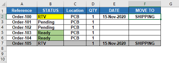
This excel file (Table) is shared among our group for updating.

Column A shows the list of our Reference Orders.

Once the Order goes out in our area, we need to Key-in the "DATE" and "MOVE TO" in columns E and F respectively.

Then, we need to manually delete the Location (PCB) in column C and then highlight the row from A to F with Grey color, and then Save.

So, when someone saves his copy on his PC, it will be updated for the latest status.

This is my question:

Is there a way that when anybody will key-in the "DATE" and "MOVE TO", it will automatically delete the Location "PCB" and then highlight the row from A to F with Grey Color and then Save? (same as the one shown in Row 7).

By the way, the MOVE TO column is normally empty. And it can be filled-up with any TEXT such as, SHIPPING, WAREHOUSE, STOCKS, MRB TEAM,, etc., etc... once we move the Order..

Hopefully, somebody can help me.

Thanks a lot in advance..

Regards,,

Rico.

Answer 1

Yes, in the steps I provided, You need to selected the affected cells. In your case if this is 200 rows, you select $A$2 to $F$201.

The formula "=AND($E2<>"",$F2<>"")" will automatically recompute in this case since the "$" is only applied in the columns E and F but not in the row number.

In the screenshot below, the one in red box will need to be changed based on the number of rows you have.

Answer 2

Hi rico_686. I’m RN, an Independent Advisor and Microsoft user like you.

I'm sorry to hear about this issue.

Is the value of column C is always "PCB"?

So that I can advise if do we need to use VBA script or formula.

Answer 3

Hi, RN

Thanks for the quick reply.

Yes. The value of column C is always "PCB".

Regards..

Answer 4

For the column C, you can use the formula below and drag the formula to all the affected column cells.

=IF(OR(ISBLANK($E2),ISBLANK($F2)),"PCB", "")

To fill the row with grey color, you need to apply conditional formating.

1. Select the affected cells (A to F)
2. Go to Home > Conditional Formatting.
3. Select New Rule
4. Select rule type "Use a formula to determine which cells to format"
5. Input formula below.

=AND($E2<>"",$F2<>"")

6. Click Format then go to fill tab.
7. Select the color you prefer then click OK
8. Click Ok
   

Answer 5

Hi, RN

I have tried the above method and it works...

I just have another concern:

For the filling-up of Grey color, I need to select the affected cells (A to F), and proceed with Conditional Formatting, then input =AND($E2<>"",$F2<>"").

This is OK if we start from a blank sheet, bec. we can just copy/drag the formatting from top to bottom.

But, in my case, I already have an existing file of around 200 rows. (So, sorry if I didn’t mention earlier)..

So, I cannot apply the formula =AND($E2<>"",$F2<>"") to all the rows. Otherwise, I have to do it one by one.

Is there an alternate way to do this?

Thanks..