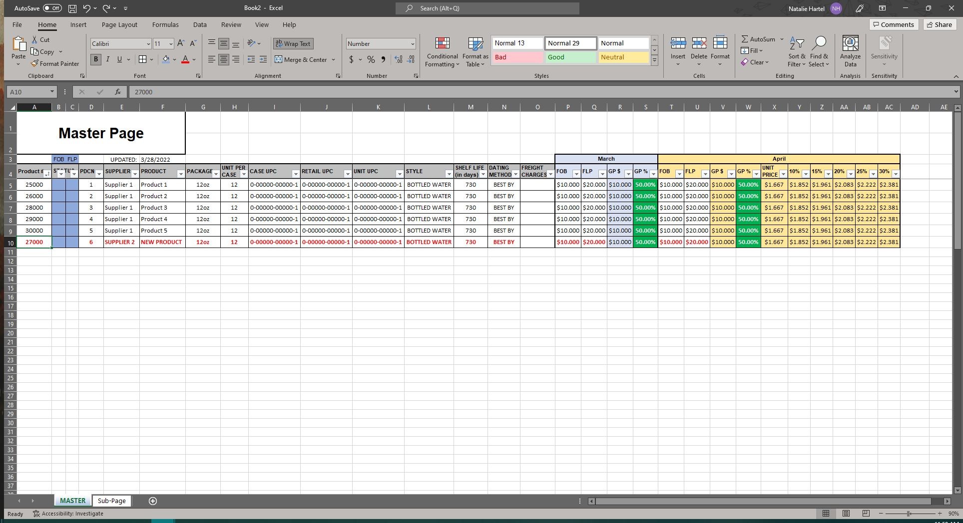
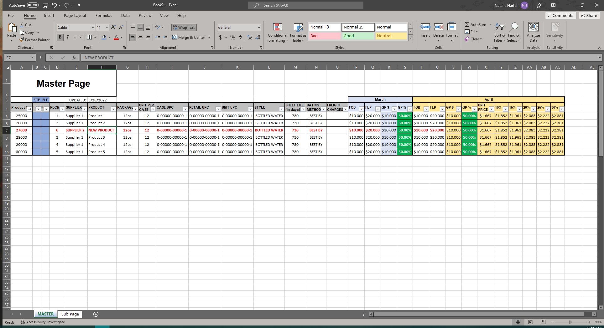
I have two sheets in the same workbook. The first is the Master sheet, where all information is input as just normal information, no formulas (except the highlighted cells, but those are just calculations on this sheet). See screenshot below.
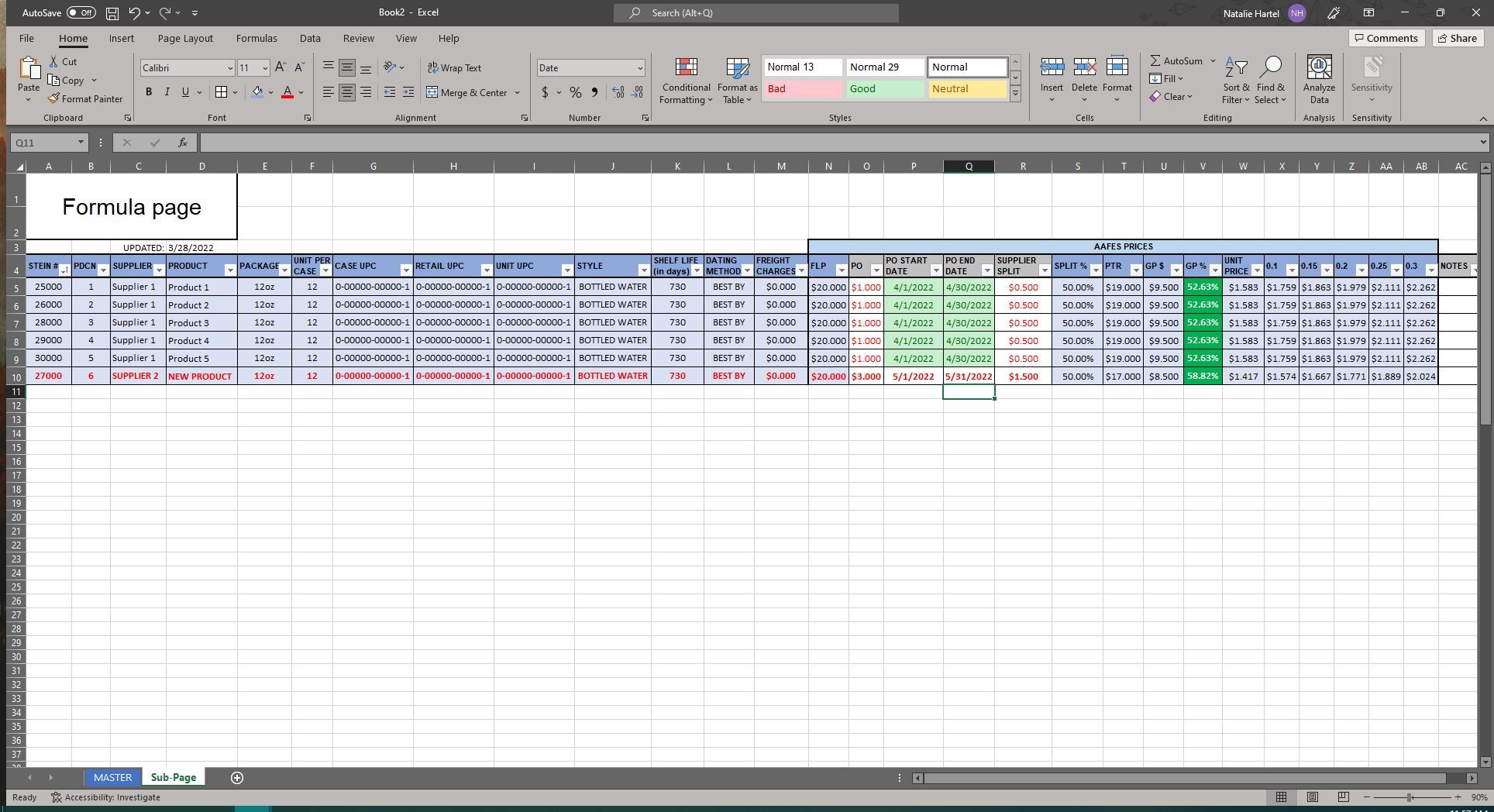
The second sheet is the Sub-Page. Here, column A is a straight ='s formula that references the Product Number in column A on the Master sheet. Columns B-N are VLOOKUPS that reference Sub-Page's column A to pull in information from the Master sheet. Columns O-R and AC are values that I input (no formulas) and columns S-AB are calculation formulas (no VLOOKUPS). See screenshot below.
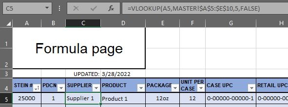
Here's a screenshot of the VLOOKUP in column C. All the VLOOKUPs have this same $ formatting.
I want my values in columns O-R and AC to stick with the products in their same rows (27000 SHOULD keep it's $3.00 PO value). I can sort the Formula page by column A and these numbers will all move around like they are supposed to. See below.
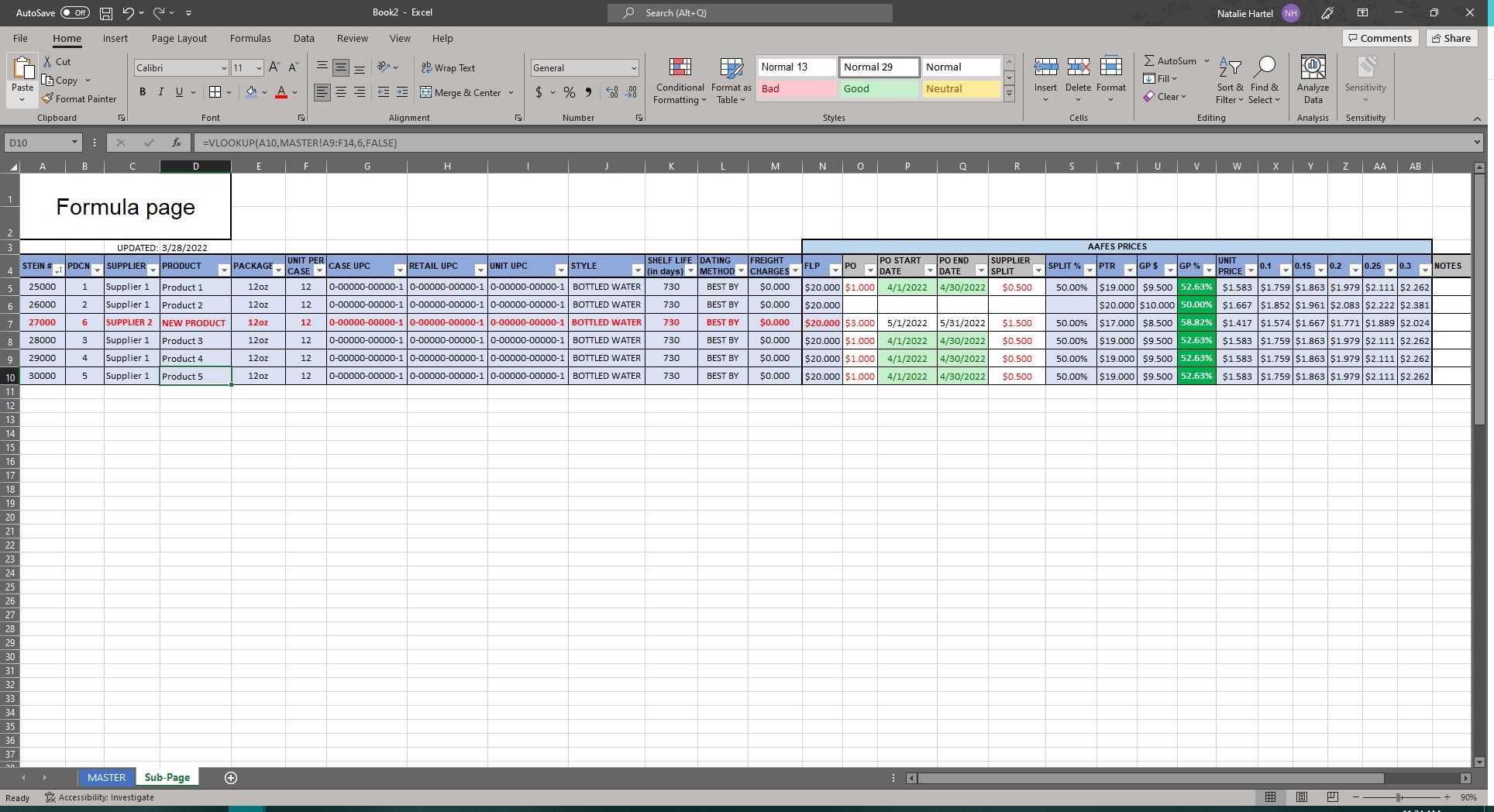
The problem that I have is when I go to sort the Master sheet by column A, the values in the Sub-Page's columns O-R and AC DO NOT stick with their correct products. Below is the screenshot of the sorted Master sheet; you can see that the "New Product" has moved into it's correct smallest-to-largest configuration:
BUT on the Sub-Page, you'll see that the formula values have shifted to correspond with the new-order on the Master-page, but the values in columns O-R have not moved with their correct products (Product 5 now has the $3.00 PO value).

How do I fix this??
