Excel Conditional Formatting using a "named range"

Question

.

End result I want:

to automate (using conditional formatting?) applying colors to dates in Col A and B when I update the dates:

So I edit formula A45 to change from = -1 + Week_1A +5 to = -1 + Week_1B +5

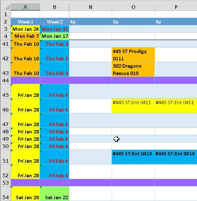
The dates in A45:A52 all change to Fri Feb 11

I want cells A45:A52 all to change from Yellow to Orange

If you can suggest a "neater" way of doing this date color management I'm open to suggestions.

.

PS: yes the -1 in the formula is a Kludge / "fudge factor", because the first day of the week does not match my internal calendar <G>.

Yes, I know I could change the system start of week, I just don't feel like it.

.

Here is a stripped down example file: https://1drv.ms/x/s!AlV7uGd6SkRXgU0B_Pz9vbnVrWyr

.

Part 1:

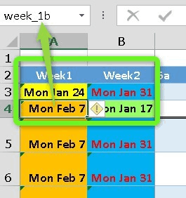
Cell A4 has been given Name "Week_1b"

Cell A5 refers to it in formula: =week_1b

Cell A16 refers to it in formula: =-1 +week_1b+2

Is there a way I can use conditional formatting to apply background color when I change formulas cells containing reference to "week_1b".

.

Part 2:

The first entry for day of week, ie A45 refers back to names in A3:B4. A45 also has a name, ie "Fri_1"

Cells A46-A52 have formula that refers to name in a45, ie a46 formula is "=Fri_1"

The effect is when I change cell A45 from "Week_1a" (yellow) to "Week_1b" (orange) all of the dates in A45-A52 change to Mon Feb 7.

But, the color remains "yellow".

When I change the color in A45 (either using CF in Part 1 of this question" I want to automatically change color in A46-A52 to match

.

Context:

Using the named cells A3:B4 I apply colors to detail content to identify "This Week", "Next Week" and "2 Weeks out", potentially "Last week".

Each day I update the previous day cell to point to "2 Weeks out"

So, in this example,

• A3 "Yellow" is "this week"
• B3 "Blue is "next week"
• A4 "Orange is "2 weeks out"
• B4 "Green" is "last week" (oops, I've been slow updating the date cell B54)

Answer 1

For any cell with a date, no matter how it is created (formula or direct entry) you can use the Formula option of Conditional Formatting to highlight the wewks as you decribe by applying 3 different levels of CF (and one base formatting for, say, the current week)

Use formulas like this for Last Week =WEEKNUM(A5)=WEEKNUM(TODAY()-7)

Use formulas like this for Next Week =WEEKNUM(A5)=WEEKNUM(TODAY()+7)

Use formulas like this for 2 Weeks out: =WEEKNUM(A5)=WEEKNUM(TODAY()+14)

Of course, change the A5 to the first cell of the selection that you are formatting with CF. You may need to use your little offset trick to get the dates "aligned" the way you want.

Note that you can change your formula:

=-1 +week_1b+2

to

=week_1b + 1