How to combine duplicate rows into one (keeping unique data only)

Anonymous
2021-12-02T12:52:38+00:00

Dear experts,

I have a list with thousands entries, first column has duplicate values, while values in the second column are different.

What I am trying to achieve is shown in the screenshot below:

  1. Column 1: To merge unique values only and omitting duplicates.
  2. Column 2: Combine data from those duplicate rows into one cell, separated by comma.

Is there a function in Excel to achieve this, can Power Query do this?

I do appreciate your kind support.

Microsoft 365 and Office | Excel | For business | Windows

Locked Question. This question was migrated from the Microsoft Support Community. You can vote on whether it's helpful, but you can't add comments or replies or follow the question.

0 comments No comments
{count} votes
Answer accepted by question author
  1. HansV 462.4K Reputation points MVP Volunteer Moderator
    2021-12-02T14:39:23+00:00

    Don't format the data on the right as a table.

    Enter the following formula in D5:

    =UNIQUE(Table1[Key])

    where Table1 is the name of the table on the left. The formula will automatically spill to the cell(s) below.

    In E5, enter the formula

    =TEXTJOIN(", ",TRUE,IF(Table1[Key]=D5,Table1[Data],""))

    and fill or copy down.

    39 people found this answer helpful.
    0 comments No comments
Answer accepted by question author
  1. Ashish Mathur 100.8K Reputation points Volunteer Moderator
    2021-12-02T23:52:27+00:00

    Hi,

    You may refer to 2 solutions in this workbook - Query Editor and formulas.

    Hope this helps.

    27 people found this answer helpful.
    0 comments No comments

6 additional answers

Sort by: Most helpful
  1. Anonymous
    2021-12-02T15:31:08+00:00

    Sir,

    I am very impressed. This has actually solved the exact problem I have.

    Thanks.

    Best Regards,

    Fares ALABED

    0 comments No comments
  2. Anonymous
    2021-12-02T15:52:53+00:00

    Hi,

    The solution provided by HansV MVP requires You to have an Office 365 subscription OR MS Excel 2021 version.

    In case You do not have the above MS Excel versions, please consider following suggestion:

    Step 1) Table name is SourceData.

    - I created a helper column - column C in screenshot below.

    -- In cell C2, please write the following formula: **** =IF(COUNTIF($A$2:A2,[@Key])=MAX(COUNTIF([Key],[@Key])),"",", ")

    - Please drag the formula down to more rows.
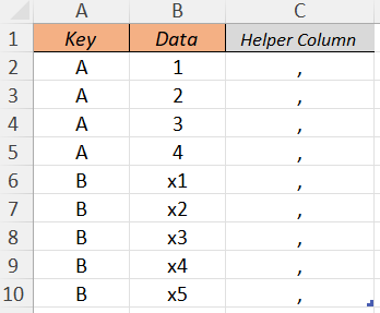
    Image

    - This helper column can be anywhere else OR can even be hidden after Step 1.

    Step 2) In cell E2, please write the following formula:

    =IFERROR(INDEX(SourceData[Key],MATCH(0,INDEX(COUNTIF($E$1:E1,SourceData[Key]),0,0),0)),"")

    - Please drag the formula down to more rows.
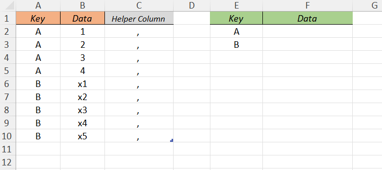
    Image

    Step 3) In cell F2, please write the following formula:

    =IFERROR(TRIM(CONCAT(INDEX(INDIRECT("B"&MATCH(E2,SourceData[Key],0)+1&":C"&MATCH(E2,SourceData[Key],0)+1+COUNTIF(SourceData[Key],E2)-1),,))),"")

    - Please drag the formula down to more rows.
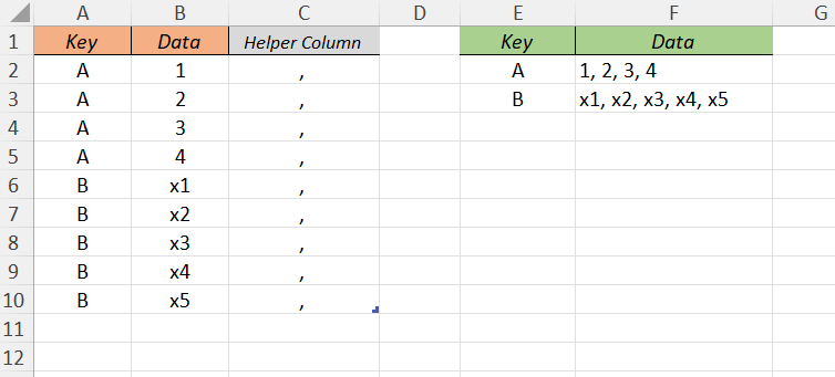
    Image

    Please respond if You require further assistance. I will try My best to be of help.

    If I was able to help You, please mark My response as answer and helpful.

    Thank You!

    11 people found this answer helpful.
    0 comments No comments
  3. Anonymous
    2021-12-02T15:54:15+00:00

    Oh . . I am sorry.

    By the time I posted My answer, it was already resolved.

    0 comments No comments