Excel 365 Version 2205 - Scatter Plot will not Display Date as the correct date on x axis with data being both in date format or text format

Question

Hello!

1. In one column I have date serial numbers. Ex. 44575
2. I use a pre set up formula in a separate column to convert it to a date : =IF(AND(A2<>0,ISNUMBER(A2)),TEXT(A2,"m/d/yyyy"),""). Ex. 01/14/2022
3. I have a third column that has found the number of times this date appears in a list
4. I then go to make a Scatter with Straight Lines and Markers.
5. For Data Select, I select the entire column of dates (step 2's column), hold control on the keyboard, and select the entire column for the number of times each date was found. (This does include fields that are currently blank incase someone wants to enter in more dates and the chart can just auto update with the new inputs)
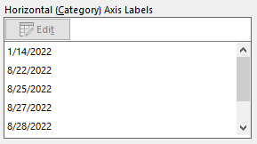
6. In select data, the dates display correctly.
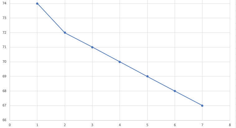
7. Once I complete the scatter, the x axis is converted to general numbers automatically showing 1,2,3,4, and not the actual dates. It displays correct like it recognizes its a time-scale and is showing the numbers corresponding to each specific date in order, it just won't display the dates properly.

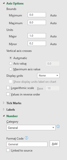
8. If I right click the horizontal axis, click Format Axis, go to "Axis Options" it shows:

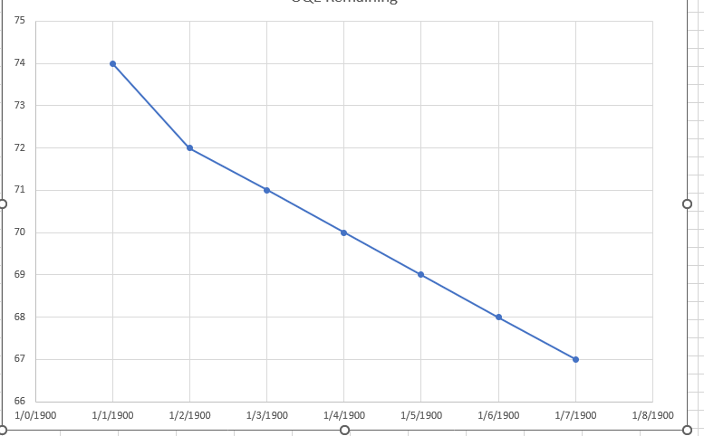
If I change format code to date, then it displays the 01/01/1900...instead of the 01/14/2022 date shown in the select data image.

Throughout this whole process, the "Select Data" pop up still displays the correct list of dates.   

How do I get my list of dates to show up properly on the x axis? Version of Excel in the title.

P.S. I did go back and mak ea column with just the dates formatted as dates and not text and used that column in the data and the samething happens. When I select "Text" in the format type, it still just displays 1,2,3,4 etc.

Answer 1

For an XY Scatter chart, ALL x-values must be numbers (including dates), without exception.

"" is not a number but a text value, so the chart uses sequence numbers 1, 2, 3, ... instead.

I'd format the first column (the one with 44575 etc.) as dates, and use that for the x-values of the chart.

Answer 2

Thank you so much, that worked! I didn't understand that it was the "" being read as a text value that set off the sequence numbers.