Exponential Regression using LOGEST

Question

I have two columns of data:

x	y
1	0.8
1200	0.5
3000	0.25
18000	0.11
45000	0.08
150000	0.05

I would like to use the LOGEST function to calculate y-values for a new set of x-values, such as:

x
1
500
1000
15000
50000

Unfortunately, just using the LOGEST function on the two columns ("=LOGEST(B2:B7,A2:A7,FALSE,FALSE)"), I get

0.99997555	1

This does not even fit the data points I already have.

Answer 1

LOGEST only returns the coefficients of the exponential trendline.

The function you're looking for is GROWTH:

=GROWTH(B2:B7,A2:A7,D2:D6)

where D2D6 contain the new x-values.

If you don't have Microsoft 365 or Office 2021, confirm the formula by pressing Ctrl+Shift+Enter.

Answer 2

Excel 365 Pro Plus

With external curve fitting.

R^2=0.9983

https://www.mediafire.com/file_premium/w76z9nn3pjwdulw/11_05_23.xlsx/file

https://www.mediafire.com/file_premium/thdeeh428y0u7xm/11_05_23.pdf/file

Answer 3

LOGEST only returns the coefficients of the exponential trendline.

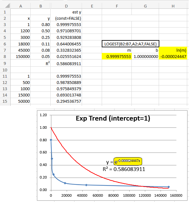
Not exactly. The LOGEST formula is y = b*m1^x, whereas the exponential trendline formula is y = b*EXP(m2*x)

The relationship between m1 and m2 is: m2 = LN(m1). Conversely, m1 = EXP(m2).

This is demonstrated below.

---

The function you're looking for is GROWTH:

=GROWTH(B2:B7,A2:A7,D2:D6)

Or more simply, the single-valued function =GROWTH($B$3:$B$8, $A$3:$A$8, A3, FALSE) in D3, for example.

That can be copied (spilled?) into D3:D8 and into D11:D15.

I prefer the single-valued form not only for its flexibility (the new values do not need to be contiguous), but also because it is difficult to change the number of cells in an array formula, at least in versions of Excel before Excel 365 and Excel 2016.

(And note the correction: the additional FALSE parameter, which is consistent with the OP's intention to force the intercept ("b") to 1.)

Answer 4

Thanks, Joe!