How to perform AVERAGE function of cells remaining *after* filtering? ie How to define new endpoints if Filter removes certain cells?

Question

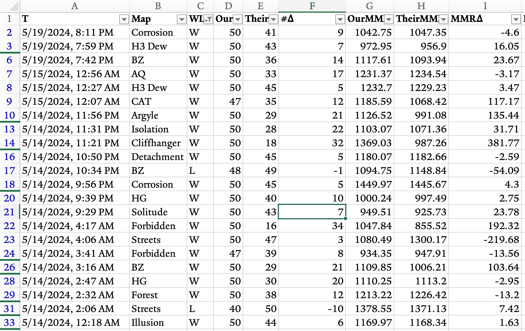
I want to conduct the AVERAGE of the Last (Most Recent) 25, Last 50, Last 100 cells, & so on both of columnF & columnI ("'I' for 'Igloo'").

Normally, in an unfiltered spreadsheet, I could simply do AVERAGE(F2:F26) for the Last 25 cells in columnF.

However, after FILTER removes certain cells, AVERAGE(F2:F26) still outputs the same average as if the spreadsheet were still unfiltered.

1. How do I take the average of the Last 25, Last 50, Last 100...Last 5000 of the new post-FILTER sheet?
2. I also want to conduct the same averages of the Last 25 (etc) on columnI. Right now, I've typed the following in a separate Word document: =AVERAGE(F2:F51) =AVERAGE(F2:F76) =AVERAGE(F2:F101) =AVERAGE(F2:F201) =AVERAGE(F2:F501) =AVERAGE(F2:F1001) =AVERAGE(F2:F2001) =AVERAGE(F2:F4001) I then paste that back into Excel. I then go back to Word to Find&Replace "F" with "I," & paste the result back into Excel. Can I accomplish that more efficiently if I'm just repeating the same function 8 or 16 times & the only thing I'm changing each time is the cells defining my endpoints (eg F2:F26...F2:4001...I2:I4001)

Answer 1

You may use subtotal function.

SUBTOTAL function - Microsoft Support

For the function_Num constants from 101 to 111, the SUBTOTAL function ignores values of rows hidden by the Hide Rows command. Use these constants when you want to subtotal only nonhidden numbers in a list.

=SUBTOTAL(101,F2:F51)