How to do INDEX MATCH in table with multiple matches

Question

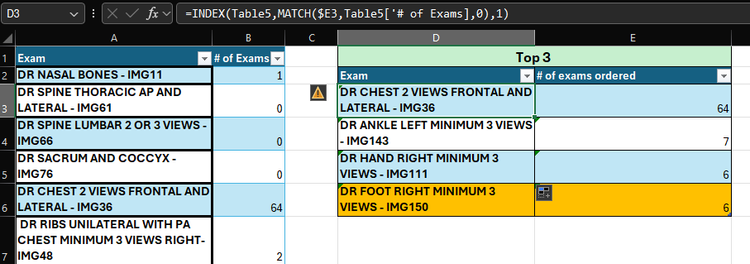
Hi, I am trying to create a table that is basically showing the top 3 results from a another table with 2 columns. However, I've been running into an issue when the values are the same, as it is only returning the first result. I need this table to automatically update monthly when I Change the data in the main table, so my top 3 results may change to more than 3 rows (like say there is two ties, one for first and two for third totaling 5 rows).  Is this possible to do using the current formula I have been using, INDEX MATCH, or is there a different formula?  I tried the FILTER function, and that returns the correct values, however I can't make it into a table. Ideally I'd like to keep my table, but if it's not possible then I will have to change it to a range. I really need this function to work, as It will be time consuming to go through the data to see if there is any tie breakers and have to manually update my top 3 results. I have figured out how to show the second result in a tie breaker, but as I've said above, I need this to automatically add or delete rows from my top 3 results table when the main data is changed, so if I'm showing the results for the top 3, I don't have to go through my main data to find a tie breaker and then have to manually add those rows to the table.  The formula I have in D3 is =INDEX(Table5,MATCH($E3,Table5['# of Exams],0),1) and the only thing that changes for D4 &D5 is the row number in my match formula, so $E4 & $E5.

The formula I have in E3 is =LARGE(Table5['# of Exams],1) and the only thing that changes for E4 & E5 is the last numbers to 2 and .

however for this data I noticed that there is a tie breaker so in cell D6 I have the formula as =INDEX(Table5,MATCH(E5,Table5['# of Exams],2),1). which returned the second result in my table.

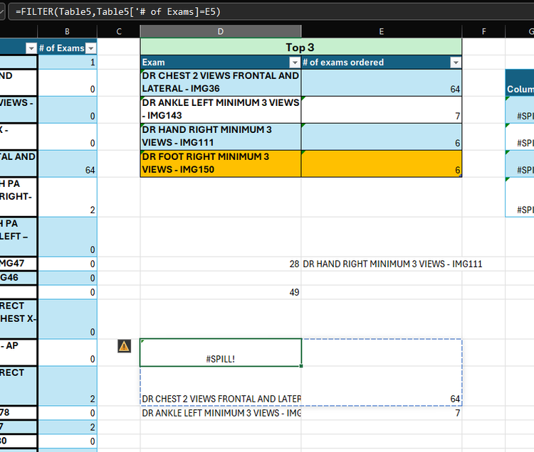
However I did try =FILTER(Table5,Table5['# of Exams]=E3), but if the data set is more then 3 rows, then It says Spill and It's the same problem as above, I need it to automatically add rows so that all my results can be shown.

I've been trying to play around with a fix, but nothing is working

I'm not sure if a power table or somethin might be needed

Any help would be very much appreciated.

Answer 1

You want to process the entire table with one formula.

Clear all of column D and E below the first row (so that the result can spill), then enter this into cell D2:

=VSTACK(A1:B1,SORT(FILTER(A:B,ISNUMBER(B:B)*(B:B>=LARGE(B:B,3))),2,-1))

That will work with either a range or a table: if you want to convert to only using the table, then try

=VSTACK(Table5[#Headers],SORT(FILTER(Table5,Table5['# of Exams]>=LARGE(Table5['# of Exams],3)),2,-1))

(This assumes that your table is still named "Table 5")

Answer 2

Hi,

Share the download link of the MS Excel file. Show the expected result there clearly.

Answer 3

https://wellstreet-my.sharepoint.com/:x:/p/abork/EdHhcIn3TAdKsR4vxEBEwv0BI1L3F8-DRsm82bKNJZVCow?e=HFaU2G

Here is the link to my document. I incorporated the formula

=VSTACK(A1:B1,SORT(FILTER(A:B,ISNUMBER(B:B)*(B:B>=LARGE(B2:B54,3))),2,-1))

It does work, however I'm not able to create a table out of it. Also my Table that I'm pulling data from for my Top 3, has a total sum of all data at the end, I had to move it over to column C so that it wouldn't be included in the above formula. Is there any way that a new formula could be created fix this?

Also, the formula returns the top 3, however, is there a way to include the top 3 results even if there is a tie for 1st and 2nd?

Answer 4

https://wellstreet-my.sharepoint.com/:x:/p/abork/EdHhcIn3TAdKsR4vxEBEwv0BI1L3F8-DRsm82bKNJZVCow?e=HFaU2G

Here is the link to my document. I incorporated the formula

=VSTACK(A1:B1,SORT(FILTER(A:B,ISNUMBER(B:B)*(B:B>=LARGE(B2:B54,3))),2,-1))

It does work, however I'm not able to create a table out of it. Also my Table that I'm pulling data from for my Top 3, has a total sum of all data at the end, I had to move it over to column C so that it wouldn't be included in the above formula. Is there any way that a new formula could be created fix this?

Also, the formula returns the top 3, however, is there a way to include the top 3 results even if there is a tie for 1st and 2nd?