How can make table filter dynamically update columns to include base on a calc/input from another cell

Question

What I'm trying to do is have a filter be dynamically edited as far as columns to include and not include various columns based on a given cell that determines weather the column should be included or not.

=FILTER(Table1[[#All],[Column1]:[Column5]],{1,0,1,0,1}) ----->would include columns 1,3 and 5 I'd like to have it so the "{1,0,1,0,1}" is determined by cell outside of the function or tabulates the columns to be included internally

Answer 1

You could enter the values 1, 0, 1, 0, 1 in 5 cells in a row. For example in K1:O1. You can then use

=FILTER(Table1[[#All],[Column1]:[Column5]],K1:O1)

A variation:

Enter the formula ={1,0,1,0,1} in K1, and use

=FILTER(Table1[[#All],[Column1]:[Column5]],K1#)

Answer 2

Hi,

You can use a combination of CHOOSECOLS() and FILTER() to get your desired result.

=choosecols(filter(A2:F100,B2:B100="A"),xmatch(H1:J1,A1:F1))

Enter this formula in cell H2. H1:J1 has the headings that you want to see in the result. A1:F1 has the headings of the source data range.

Hope this helps.

Answer 3

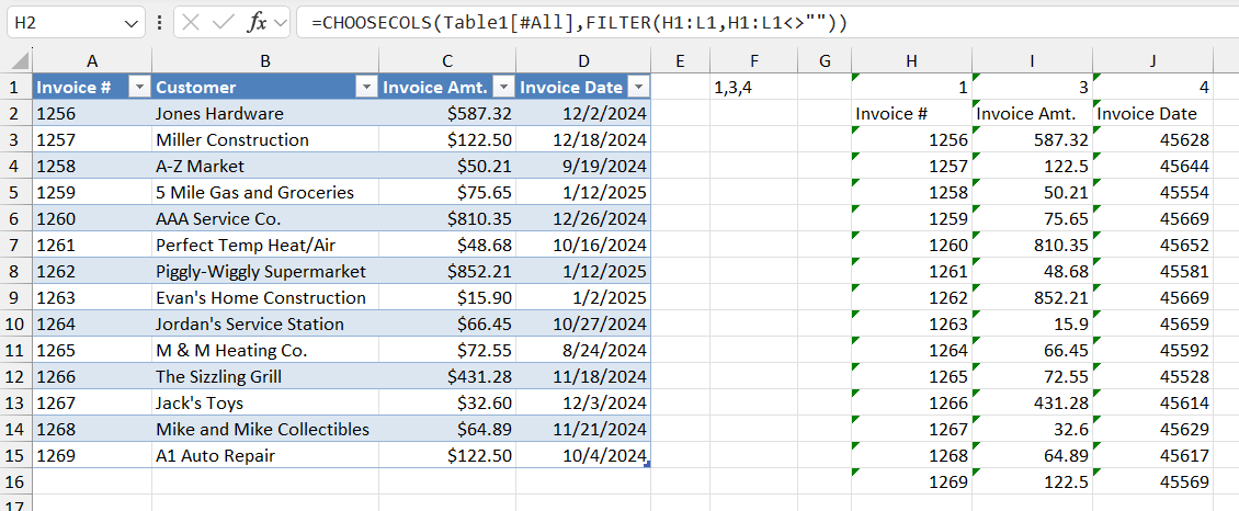
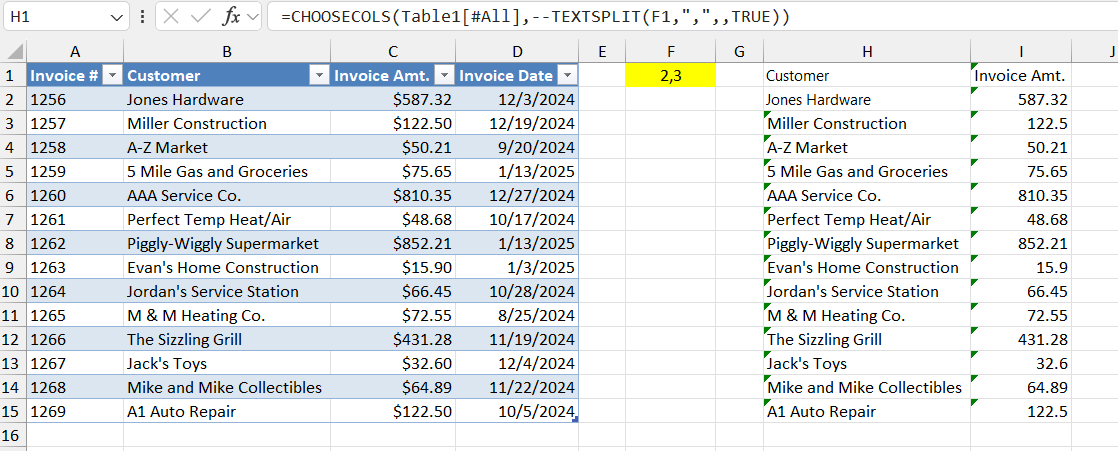
Here is a screenshot with explanations below that will allow you to filter the table with a one cell list of the columns that you want. These could be typed in a cell or pulled up using Data Validation for specific combinations.

*F1 is the location of the desired columns list. This could be typed in, use a VLOOKUP to retrieve, or chosen from a Data Validation list.

*H1 is this formula to separate the column numbers in F1 so the CHOOSECOLS function will recognize them. This will split however many columns there are in the list in F1 into separate columns.

=--TEXTSPLIT(F1,",",,TRUE)

*To filter the Table into only the desired columns, use this formula. I have it in H2 in the screenshot. The FILTER part of the formula is matching the column list from the TEXTSPLIT function to the same number of column numbers that are listed in F1 so that it is flexible for different numbers of columns. I used H1:L1. Make this range large enough to accommodate the maximum number of columns you will want to filter down to at any one time.

=CHOOSECOLS(Table1[#All],FILTER(H1:L1,H1:L1<>""))

EDIT: simplified

Replace the CHOOSECOLS formula above with this one. This also eliminates the need for the TEXTSPLIT formula in H1 and the FILTER function in the formula above. Simply enter the column numbers in a cell (currently F1--adjust for the location you choose) separated by commas with no spaces and enter this formula where you want to see the filtered columns from the Table.

=CHOOSECOLS(Table1[#All],--TEXTSPLIT(F1,",",,TRUE))