Hi @Shakil Nagori
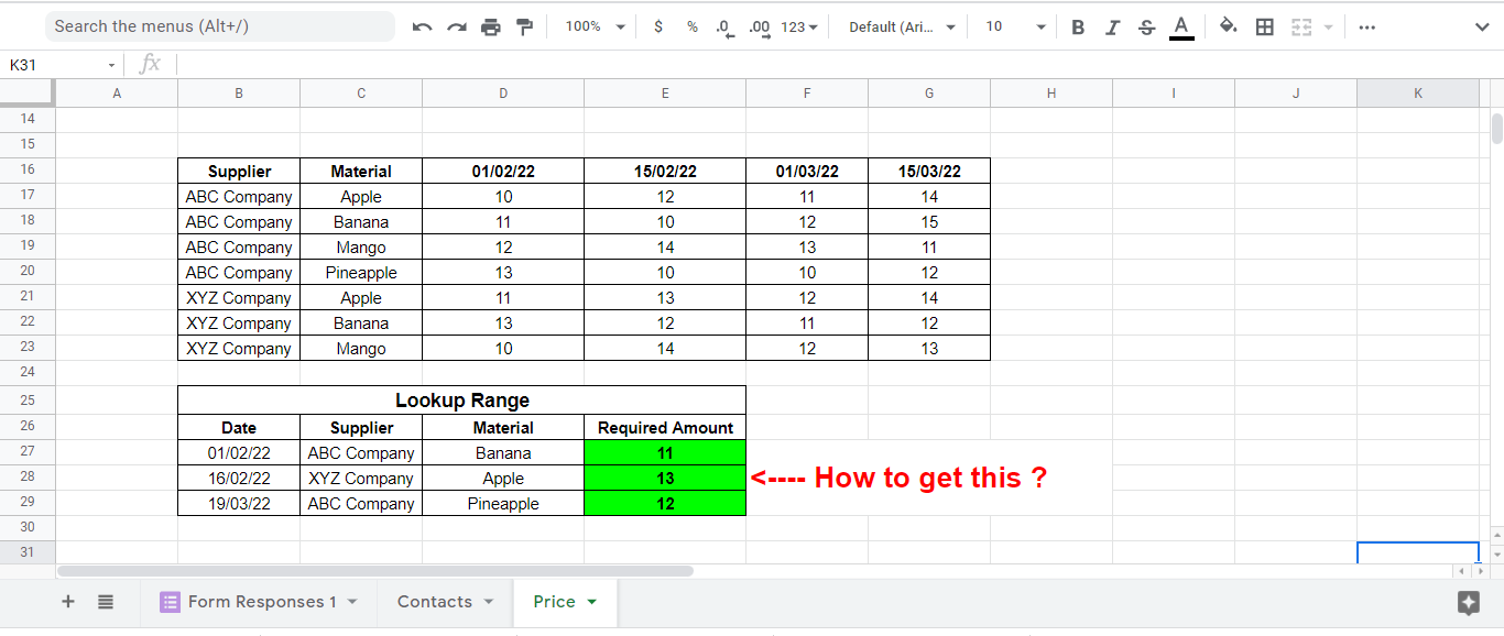
Accoring to your description, I have a question, will the date criterias and the dates of the source data be different?
If not, they are the same, please check whether Lz-3068's reply is helpful.
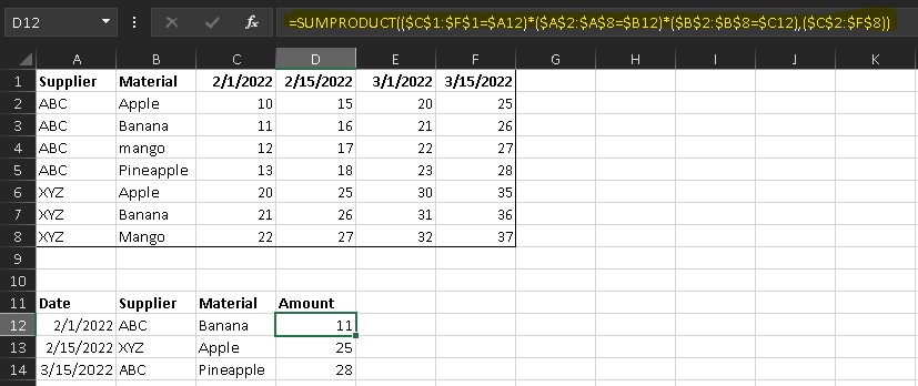
You could also try Sumproduct function, =SUMPRODUCT(($C$1:$F$1=$A12)*($A$2:$A$8=$B12)*($B$2:$B$8=$C12),($C$2:$F$8))
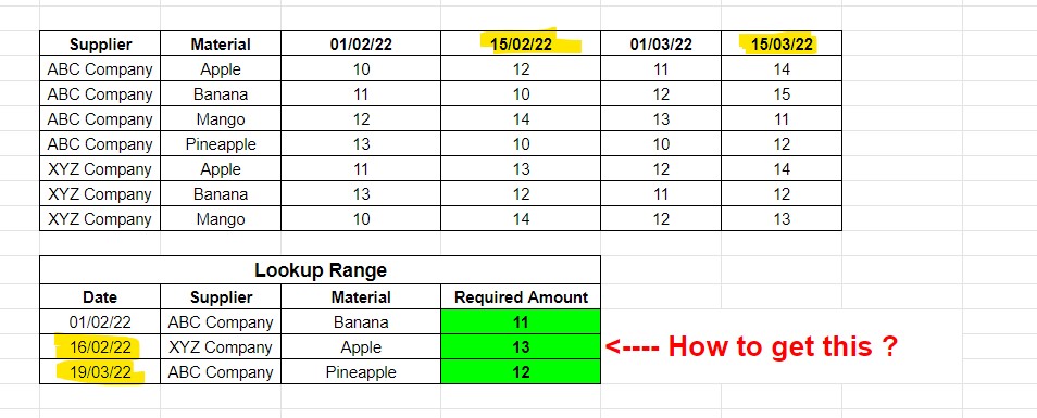
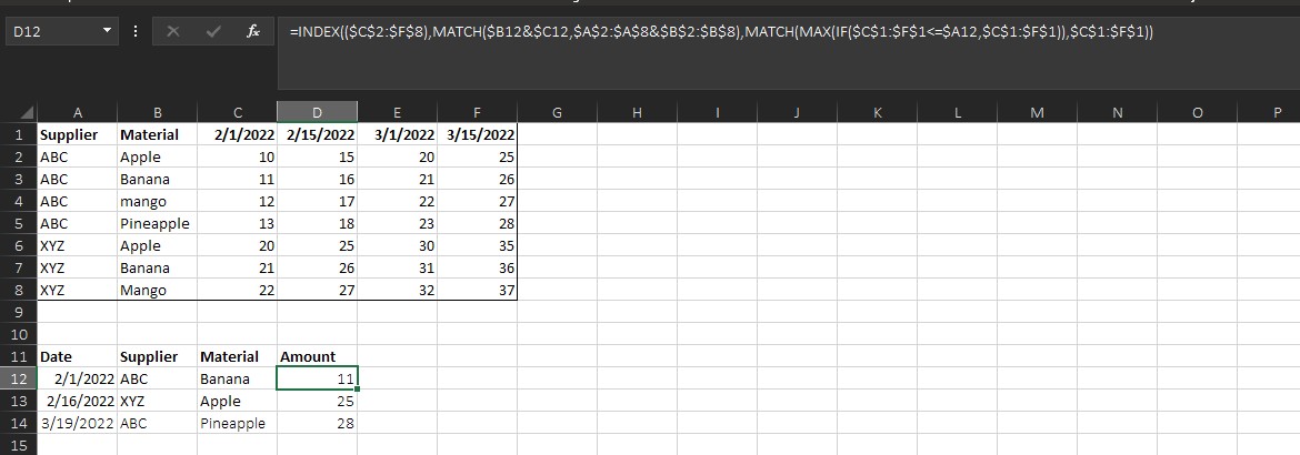
If yes, they are may not same, please try following formula.
=INDEX(($C$2:$F$8),MATCH($B12&$C12,$A$2:$A$8&$B$2:$B$8),MATCH(MAX(IF($C$1:$F$1<=$A12,$C$1:$F$1)),$C$1:$F$1))
Any updates, you can let us know.
If the answer is helpful, please click "Accept Answer" and kindly upvote it. If you have extra questions about this answer, please click "Comment".
Note: Please follow the steps in our documentation to enable e-mail notifications if you want to receive the related email notification for this thread.
' cx='32' cy='32' r='32' /%3E%3Ctext x='50%25' y='55%25' dominant-baseline='middle' text-anchor='middle' fill='%23FFF' %3ESN%3C/text%3E%3C/svg%3E)