conditional format based on text?

Question

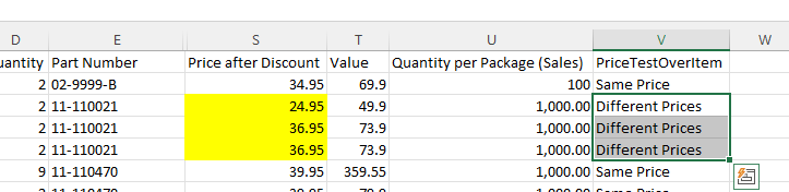
Is there a conditional format where if a certain text is written I can highlight values in another column?

Answer 1

Hi, @Jonathan Brotto
You can click New Rule in Conditional Formatting, select Use a formula to determine the cells to be formatted, and write the formula in the dialog box. The example steps are as follows:

1. Select the area where you want to highlight the cells.
2. Click the Conditional Formatting button in the Home tab, and select New Rule in the pop-up menu.
3. Bring up the New Formatting Rule window, and the "Select Rule Type" is Use a formula to determine which cells to set.
4. Enter =$B1=”NO” in the “Format values that match some formulas” box, and then click the Format button to select the desired cell format to complete the conditional formatting.
   
   In the formula you can enter the text you want.

---

If the response is helpful, please click "Accept Answer" and upvote it.
Note: Please follow the steps in our documentation to enable e-mail notifications if you want to receive the related email notification for this thread.