Conditional Formatting with an image

Question

Conditional Formatting with an image

Victor Lopez 41

Hello,

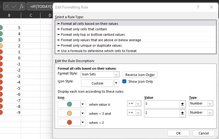
I wanted to add a conditional formatting for expiration dates. Currently I am using :

=EDATE(TODAY(),1) =EDATE(TODAY(),2) =EDATE(TODAY(),3) for 1 month out, 2 months out and 3 months out with Red Orange Green color formatting.

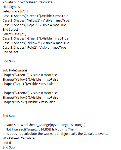
This is working fine, but I wanted to use little traffic lights instead of the color formatting. I managed to find a VBA code that brings up the traffic lights, I am using the following:

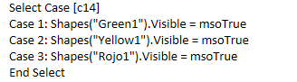
Select Case [c14]
Case 1: Shapes("Green1").Visible = msoTrue
Case 2: Shapes("Yellow1").Visible = msoTrue
Case 3: Shapes("Rojo1").Visible = msoTrue
End Select
Select Case [b5]
Case 1: Shapes("Green2").Visible = msoTrue
Case 2: Shapes("Yellow2").Visible = msoTrue
Case 3: Shapes("Rojo2").Visible = msoTrue
End Select

'etc. for all 9 cells

End Sub

Sub HideSignals()
Shapes("Green1").Visible = msoFalse
Shapes("Yellow1").Visible = msoFalse
Shapes("Rojo1").Visible = msoFalse

Shapes("Green2").Visible = msoFalse
Shapes("Yellow2").Visible = msoFalse
Shapes("Rojo2").Visible = msoFalse

End Sub

Private Sub Worksheet_Change(ByVal Target As Range)
If Not Intersect(Target, [c14,B5]) Is Nothing Then
'this does not calculate the worksheet. It just calls the Calculate event.
Worksheet_Calculate
End If
End Sub

The problem with this is, it only works if the value in the cell is 1,2, or 3. I want to make it so that it also uses date values "Today" and then the 30 days, 60 days and 90 days format. I know that the 1,2,3 comes from the value placed after the "Case" (Case #:) but i want to know if I can make that a date and how would I modify it.

Accepted answer

0 additional answers

Your answer

Answer 1

Michael Taylor 60,326

To get the # of months between 2 dates you can use this: =IF(TODAY() > $A2, -DATEDIF($A2, TODAY(),"m"), DATEDIF(TODAY(), $A2,"m")) where $A2 is just a cell reference. This would return the # of months between the given cell's date and today. DATEDIF doesn't like negative values so the IF is required. Given this formula you can then select the correct icon set using conditional formatting.

If you want to continue doing this in a script then replace the simple select case statement with select case <formula>. You then get back the # of months and can use the simple case statement.

Select Case IF(TODAY() > c14, -DATEDIF(c14, TODAY(),"m"), DATEDIF(TODAY(), c14,"m"))
Case 1: Shapes("Green1").Visible = msoTrue
Case 2: Shapes("Yellow1").Visible = msoTrue
Case 3: Shapes("Rojo1").Visible = msoTrue
End Select

If you have that value already calculated in your spreadsheet somewhere then you can use the conditional formatting UI to do the same thing. But if you don't then it becomes harder because icon sets and custom formulas don't work together so you end up having to use multiple rules.

Victor Lopez 41 Reputation points

2022-06-03T14:50:13.87+00:00

Thanks for the quick response,

I got a Syntax Error for the first line:

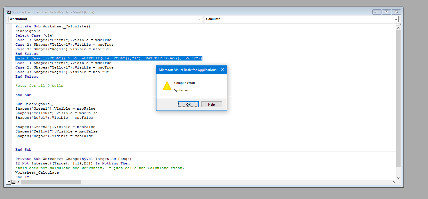
Did I do something wrong?
Michael Taylor 60,326 Reputation points

2022-06-03T15:05:38.59+00:00
Sorry I didn't translate to VB.

Change If to IIf

Add an extra paren on the end.

Select Case IIf(TODAY() > c14, -DATEDIF(c14, TODAY(),"m"), DATEDIF(TODAY(), c14,"m")))

If that doesn't work then I'll have to write a test script. This formula works in conditional formatting so it is just a matter of getting it to work with your script.
Victor Lopez 41 Reputation points

2022-06-03T15:08:43.68+00:00

So I actually managed to get it to "work" by using the formula you provided for calculating the months between todays date and the date inputed into the cell by creating another column (That i ended up hiding) and having the original VBA I used reference the hidden cell instead of the date cell. The only question I have left is how I would get "Case 1: Shapes("Rojo1").Visible = msoTrue" to reference 1 or less and "Case 3: Shapes("Green1").Visible = msoTrue" to be 3 or more.

Thanks for all the help so far this is working great, I plan on using your modified script on a test excel to see which one works cleaner
Michael Taylor 60,326 Reputation points

2022-06-03T15:22:44.767+00:00
If you need relative values then a select statement won't work anymore. You'll need to use a set of if-else-if.

Dim diff As Integer diff = IIf(TODAY() > c14, -DATEDIF(c14, TODAY(),"m"), DATEDIF(TODAY(), c14,"m"))) If diff <= 1 Then Shapes("Green1").Visible = msoTrue Else If diff = 2 Then Shapes("Yellow1").Visible = msoTrue Else Shapes("Rojo1").Visible = msoTrue End If

But if you already have a column with the calculated value then you don't really need the script anymore. You can use conditional formatting to associate the icon set with the column value and hide the value itself and just show the icon. No scripting is required.

Assume you have a column with the calculated value If(TODAY() > $c14, -DATEDIF($C14, TODAY(),"m"), DATEDIF(TODAY(), $C14,"m"))). It shows the month differences. Add conditional formatting to that column, hide the value and set the icons based upon the relative values.
Victor Lopez 41 Reputation points

2022-06-06T20:38:53.787+00:00

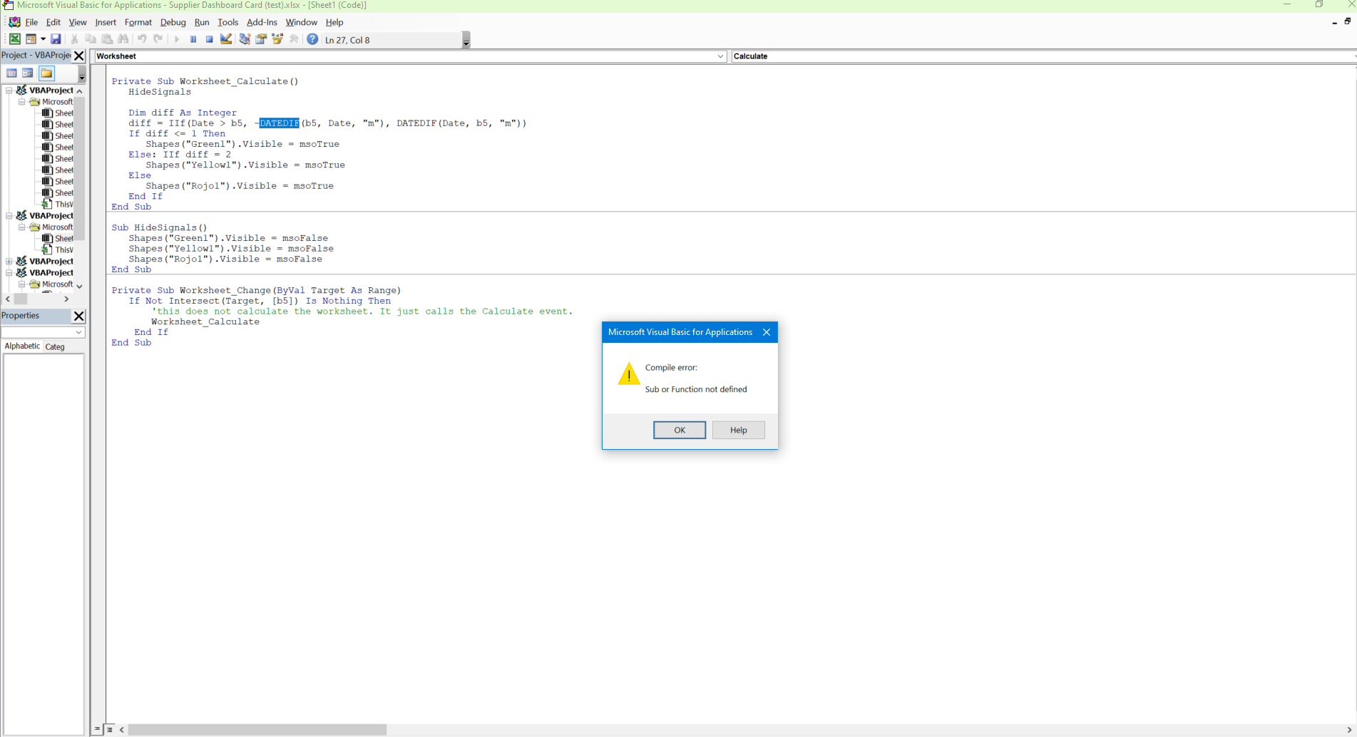
Revisiting this thread as I'm trying the if-else-if method but this is the error that I'm given. Any ideas where I may have messed up?
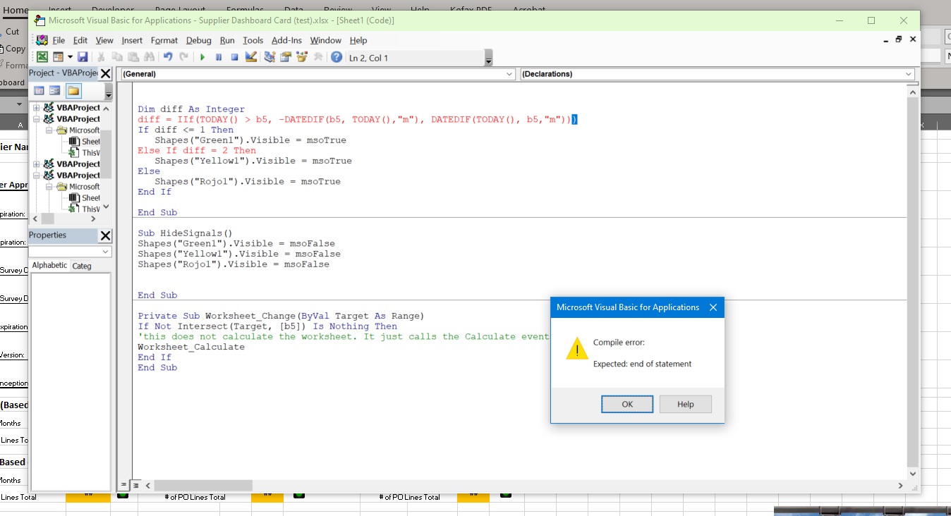
Michael Taylor 60,326 Reputation points

2022-06-06T20:49:26.863+00:00

One too many closing parens. Remove the last one and see if the error goes away.
Victor Lopez 41 Reputation points

2022-06-07T12:57:04.357+00:00

That fixed that compiling error. But it provided me with this one:

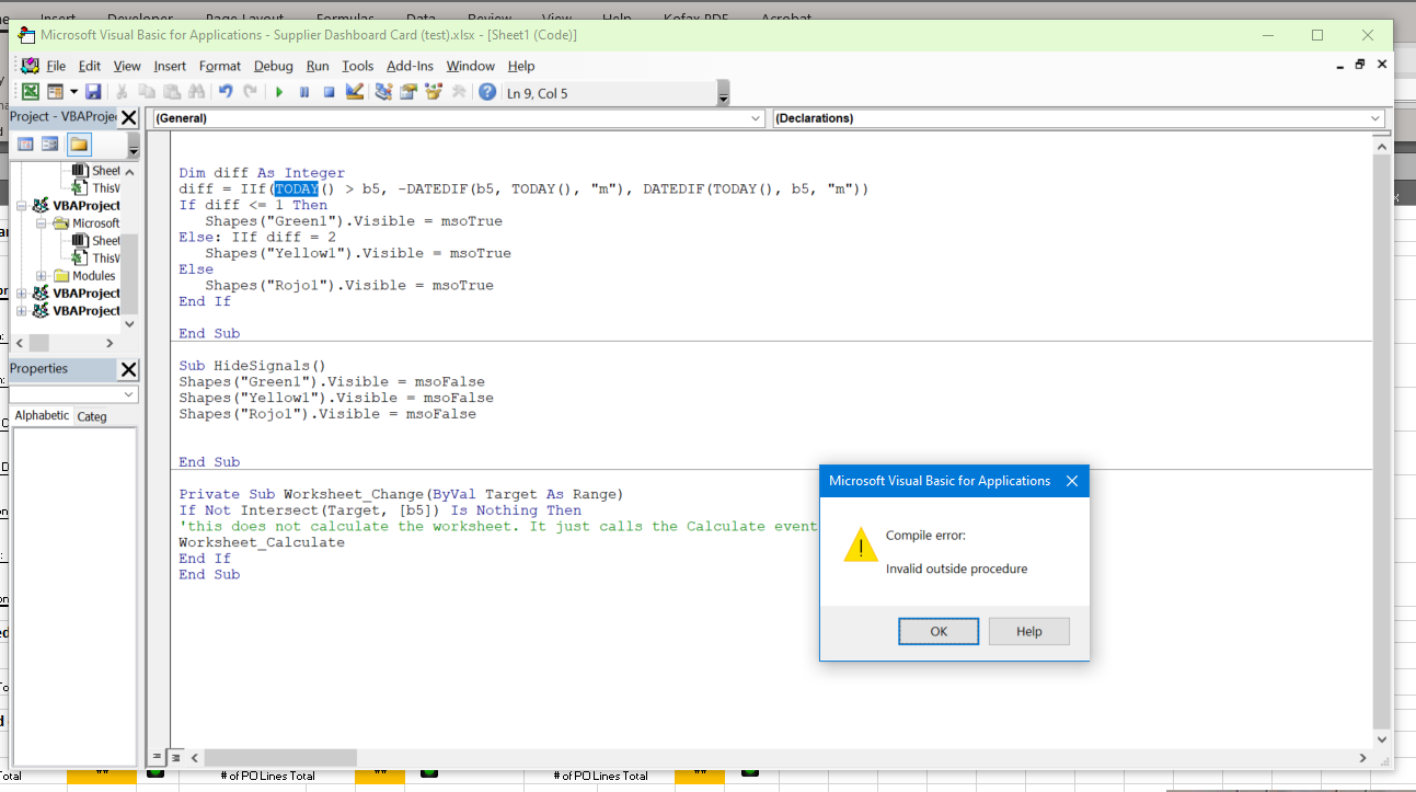
I appreciate all the help so far.
Michael Taylor 60,326 Reputation points

2022-06-07T14:13:33.17+00:00
Can you provide the entire contents of that file? Looking at the code you posted it appears you might be at the top of the file but the Dim diff code isn't inside a Sub. You have the End Sub but it looks like you might have accidentally deleted everything before the code block when you pasted it.

I believe you originally had something like this:

Private Sub Worksheet_Calculate () HideSignals() //Dim code goes here...
Victor Lopez 41 Reputation points

2022-06-07T14:24:06.913+00:00

Original code was:

So the Dim would replace the:

Correct?
Michael Taylor 60,326 Reputation points

2022-06-07T16:44:39.627+00:00

Yes I believe so. Once you've made that change, if you're still getting errors then please post the updated Worksheet_Calculate sub code.
Victor Lopez 41 Reputation points

2022-06-07T16:55:18.337+00:00

Compile Error: Expected End Sub

Private Sub Worksheet_Calculate()
HideSignals
Sub DateDiff()
Dim diff As Integer
diff = IIf(Date > b5, -DATEDIF(b5, Date, "m"), DATEDIF(Date, b5, "m"))
If diff <= 1 Then
Shapes("Green1").Visible = msoTrue
Else: IIf diff = 2
Shapes("Yellow1").Visible = msoTrue
Else
Shapes("Rojo1").Visible = msoTrue
End If

End Sub

Sub HideSignals()
Shapes("Green1").Visible = msoFalse
Shapes("Yellow1").Visible = msoFalse
Shapes("Rojo1").Visible = msoFalse

End Sub

Private Sub Worksheet_Change(ByVal Target As Range)
If Not Intersect(Target, [b5]) Is Nothing Then
'this does not calculate the worksheet. It just calls the Calculate event.
Worksheet_Calculate
End If
End Sub

Michael Taylor 60,326

You added a Sub DateDiff() in the middle of the code. Try this.

Private Sub Worksheet_Calculate()
   HideSignals

   Dim diff As Integer
   diff = IIf(Date > b5, -DATEDIF(b5, Date, "m"), DATEDIF(Date, b5, "m"))
   If diff <= 1 Then
      Shapes("Green1").Visible = msoTrue
   Else: IIf diff = 2
      Shapes("Yellow1").Visible = msoTrue
   Else
      Shapes("Rojo1").Visible = msoTrue
   End If
End Sub

Sub HideSignals()
   Shapes("Green1").Visible = msoFalse
   Shapes("Yellow1").Visible = msoFalse
   Shapes("Rojo1").Visible = msoFalse
End Sub

Private Sub Worksheet_Change(ByVal Target As Range)
   If Not Intersect(Target, [b5]) Is Nothing Then
       'this does not calculate the worksheet. It just calls the Calculate event.
       Worksheet_Calculate
    End If
End Sub

Victor Lopez 41 Reputation points

2022-06-07T19:29:44.027+00:00

Compile Error: Sub or function not defined (Directly copied and pasted your code)
Michael Taylor 60,326 Reputation points

2022-06-07T19:51:09.32+00:00
I'm not sure what happened with the code that I posted and the various iterations that you made but I can see multiple syntactical errors in the code that weren't in the original version. However the code you're posting is relying on stuff that I don't have in my worksheet. Specifically the Shapes("Green1")... and b5 stuff isn't valid outside the context of your code so I don't know how to replicate that. I assume that b5 somehow represents a specific cell in your worksheet but I cannot get it to have a value. So here's a version of the code that doesn't have syntactical errors but may or may not work given your definitions of stuff that I don't have.

Private Sub Worksheet_Calculate() HideSignals Dim diff As Integer diff = IIf(Date > b5, -DateDiff(b5, Date, "m"), DateDiff(Date, b5, "m")) If diff <= 1 Then Shapes("Green1").Visible = msoTrue ElseIf diff = 2 Then Shapes("Yellow1").Visible = msoTrue Else Shapes("Rojo1").Visible = msoTrue End If End Sub Sub HideSignals() Me.Shapes("Green1").Visible = msoFalse Me.Shapes("Yellow1").Visible = msoFalse Me.Shapes("Rojo1").Visible = msoFalse End Sub Private Sub Worksheet_Change(ByVal Target As Range) If Not Intersect(Target, [b5]) Is Nothing Then 'this does not calculate the worksheet. It just calls the Calculate event. Worksheet_Calculate End If End Sub
Victor Lopez 41 Reputation points

2022-06-07T20:02:37.137+00:00

B5 is the cell that has the date on the worksheet
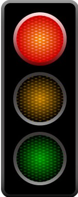
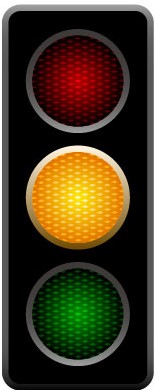
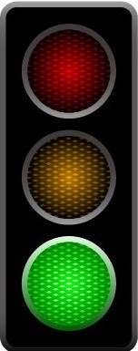
Green1 is the name of the "picture" icon, I just inserted a picture of a green stop light and named it "green1" so I had a reference in the VBA.

I've attached the images below if that may help, There was a "Run time error '13' Type Mismatch" for line:

diff = IIf(Date > b5, -DateDiff(b5, Date, "m"), DateDiff(Date, b5, "m"))

209243-green.jpeg
Michael Taylor 60,326 Reputation points

2022-06-07T20:26:03.03+00:00

That's because your b5 isn't actually a date and therefore the comparison won't work. You'll need to take a look at the data in that cell and do the conversion to a date so that the comparison can be done. Unfortunately this is dependent upon how the data is stored in the cell. If you cannot figure it out then perhaps you can attach a sample worksheet with the code and sample data that we can use as a basis for testing.

Share via

Conditional Formatting with an image

0 additional answers

Your answer