Join two excel table

Question

We have two excel files , they have the common filed ( student ID ) , I would like to join the tables so that the output as below table ( after vlookup ) , would advise what can I do ? thanks

Table 1

student ID Student Name
001 Peter
002 Tom
003 Mary

Table 2

student ID Class
001 Form 1
002 Form 2
003 Form 3

After vlookup

==============

student ID Student Name Class
001 Peter Form 1
002 Tom Form 2
003 Mary Form 3

Answer 1

Hi, @chan patrick

You can enter =VLOOKUP(B10,Table1,2,FALSE) in C10 and enter =VLOOKUP(B10,Table2,2,FALSE) in D10, and when you enter the student in B10 you can get the information from the two tables.

---

If the response is helpful, please click "Accept Answer" and upvote it.
Note: Please follow the steps in email-notifications to enable e-mail notifications if you want to receive the related email notification for this thread.

Answer 2

Hey Patrick, maybe you can prove the XLOOKUP function.
=XLOOKUP(look up value in this case you ID,Look up Array in this case the second file but only de column where there's the IDs,* Return Array in this case the second file but only de column where there's the forms for each ID*)

Answer 3

Hi @chan patrick , They are three solutions which I can proffer you use,

• Vlookup

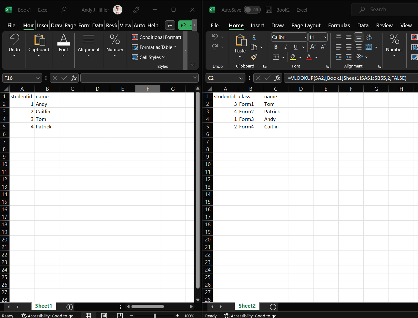
You can use the Solution offered by @Charles Qi_MSFT which states You can enter =VLOOKUP(B10,Table1,2,FALSE) in C10 and enter =VLOOKUP(B10,Table2,2,FALSE) in D10, and when you enter the student in B10 you can get the information from the two tables. If you want to use it from two different worksheets, In the argument for the Lookup range you would highlight the range in the other workbook and add lock(This could be accomplished using the fn+f4 key or f4key depending on your system) the selected range in the sheet highlighted, and you should still be able to achieve your desired result

• Xlookup
  Xlookup also performs similar function, However Xlookup has fewer arguments as @Hazel Hireki Cruz Alvarado highlighted =XLOOKUP(look up value in this case you ID, Look up Array in this case the second file but only de column where there's the IDs, Return Array in this case the second file but only de column where there's the forms for each ID), However it is important to note that Xlookup Features are available to newer Version of Excel (Came out in 2019)
• Power Pivot
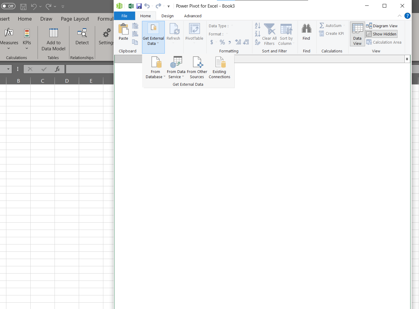
  You can use Power Pivot to connect two related tables using relationships, and you In this case the related column would be the student ID, if you are using a version of excel newer than 2010, you should have Power Pivot available to you, how you can access it is by going to the file tab, clicking on options, select add-ins, Under the manage tab, change the Excel Add-Ins to Com Add-ins, click on go, tick power Pivot and you can close the options tab once you have enabled Power Pivot, You should see the Power Pivot Tab on your Ribbon.
  For further research on how to use PowerPivot you can visit https://www.excelcampus.com/functions/powerpivot-instead-vlookup/

If the response is helpful, please click "Accept Answer" and upvote it.

Answer 4

Hi Patrick,

The easiest way to do this while still utilizing a vlookup and not SQL, OLEDB/ODBC, Power Query Tables, etc. would be to pass the name of the source data workbook into square brackets. See the below screenshot as an example, where I use [Book1] to reference the Application.Workbook object 'Book1', a different file.

Hopefully this helps!