Visualizing Climate Data in Phase Space, Part 2
I promised in an earlier post to implement a visualizer for Poincaré sections. This is a new feature for my phase-space visualizer, and it displays a cross-sectional view of a (usually) tangled phase-space trajectory. If you haven't read the first post, you might want to, or the following discussion will make absolutely no sense.
A Poincaré section is a slice through phase space. It can reveal interesting structures, called attractors , which constrain the orbits through phase space. The following diagram shows a Poincaré section with two different orbits: one is periodic and intersects a single point on the section repeatedly; the other is non-periodic and intersects at many different points.
![A Poincaré section, or map [Credits : Encyclopædia Britannica, Inc.]](https://media-2.web.britannica.com/eb-media/88/26988-004-F5AB3E80.gif "A Poincaré section, or map
[Credits : Encyclopædia Britannica, Inc.]")
A Poincaré section in phase space (Encyclopedia Britannica).
The periodic signal has a fixed-point attractor. The non-periodic signal may have one of any number of attractors. If the signal is chaotic, the attractor will appear as a fractal distribution on the Poincaré section. These are commonly called strange attractors. If everything were to come together perfectly, I'd hope to see something like the following attractors in my insolation sections:
Fractal ("strange") attractors revealed in Poincaré sections.
Keep in mind that "chaotic" does not mean random; it refers to randomlike variations that are purely deterministic, but sensitive to initial conditions. Chaotic oscillations occur in systems with nonlinear feedbacks, and Earth's climate system definitely fits this description.
In Part 1, I embedded climate data in a three-dimensional phase space and looked for interesting patterns. There were tantalizing hints of structure, but no smoking gun. The data sets generated by Dr. Raymo were too short for much detail to be visible in a Poincaré section, so I needed to generate my own.
I especially wanted to look for attractors in the insolation signal. Insolation drives Earth'[s climate system, and understanding this input signal gives us a better chance of understanding the system's response to it. In particular, if we can show that the input signal is chaotic, we can expect to find chaotic oscillations in the climate system's response.
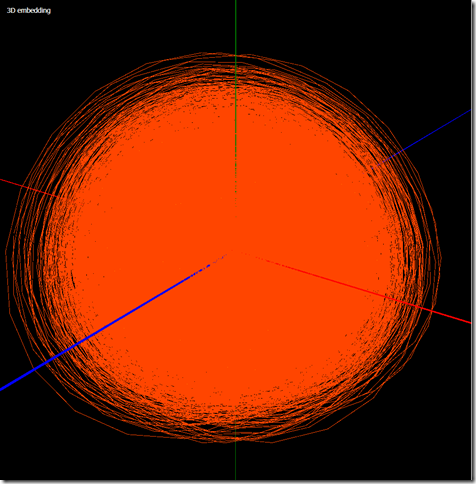
The insolation signal is generated from a mathematical model of Earth's orbital dynamics. Dr. Raymo kindly pointed me to a handy Mac implementation named AnalySeries, so I didn't have to reverse-engineer a FORTRAN implementation named Insola. To see any interesting patterns in a Poincaré section typically requires a very large data set, so I used AnalySeries to generate 100 million years of data. Data points occur at 1000-year intervals, so there are 100,000 data points. The 3D phase-space portrait with an embedding delay of 7 samples (7,000 years) looks like this:
Phase space portrait of 100 million years of insolation data.
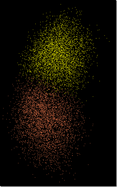
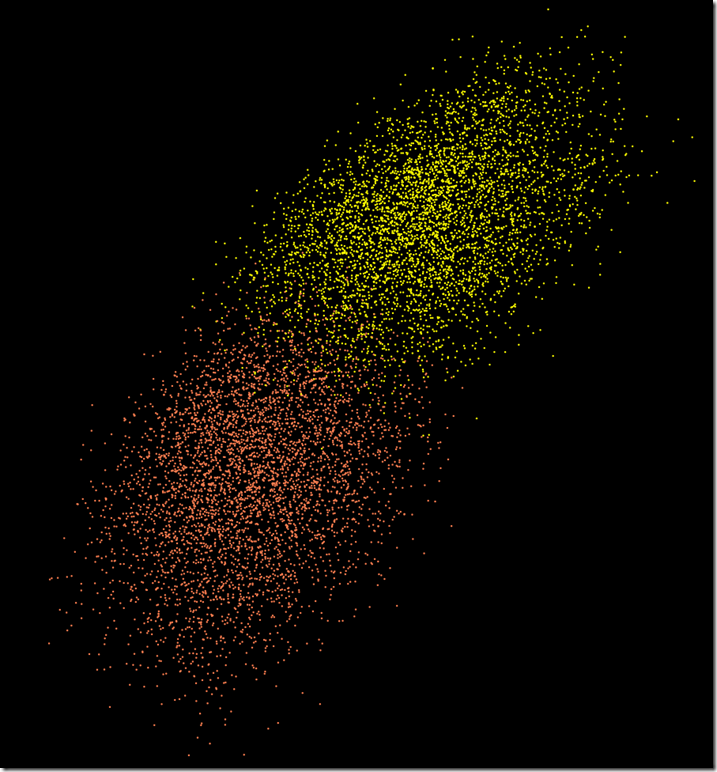
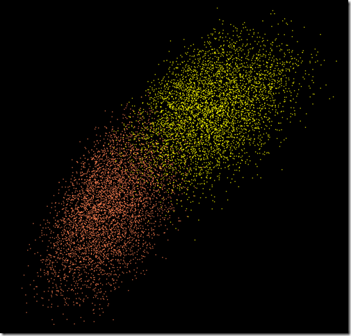
Not very helpful. But if we take a slice along the XY-plane, we may see more detail. The following images show the Poincaré sections for two phase-space portraits, with 6- and 7-sample embedding delays. Each orbit makes a dot when it crosses the plane. Downward-traveling crossings make an orange dot, and upward-traveling crossings make a yellow dot. There are 9063 crossings shown in each of the following Poincaré sections.
Poincaré sections for delays of 6 samples (left) and 7 samples (right).
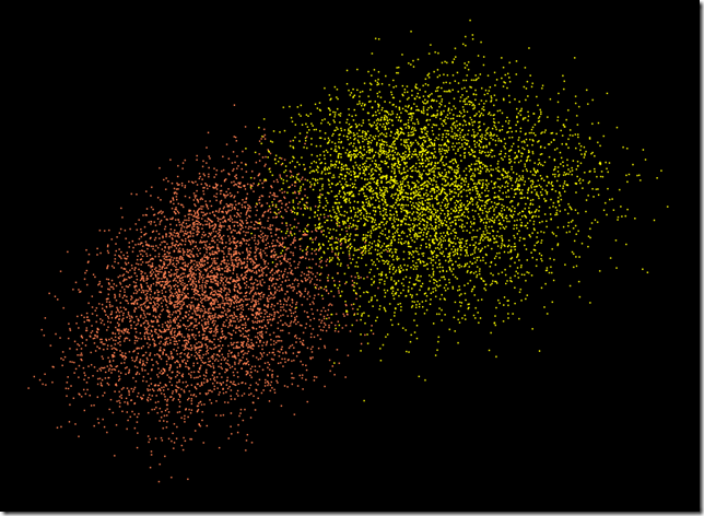
Here are the sections along the YZ-plane:
Poincaré sections along the YZ-plane for delays of 6 samples (left) and 7 samples (right).
I find these sections to be highly suggestive of fractal structure, but there's nothing as clear as in the previous example plots. A fractal attractor might be more visible with a longer data set, but unfortunately AnalySeries generates only 100 million years of insolation data.
All is not lost, however. It's possible visualize the flow by rotating the Poincaré section around an axis and animating the intersection points as it moves. This isn't hard in principle, but it requires more coding. Because the data set is so large, realtime animation is out of the question, so I need to make a WMV out of successive snapshots. That's some more coding. I'll get back to you when I have something that works.
Comments
Anonymous
June 18, 2009
PingBack from http://thestoragebench.info/story.php?id=2570Anonymous
February 09, 2013
One of your figures is captioned "Fractal ("strange") attractors revealed in Poincaré sections." What is appears in the picture are KAM curves... there is absolutely no attractor there.
