New book: Visual Models for Software Requirements

We’re happy to announce that Visual Models for Software Requirements (ISBN 9780735667723; 480 pages) is now available for purchase! Written by Joy Beatty and Anthony Chen—experts in software requirements methodologies—this book provides IT business analysts a plethora of best-practice techniques on how to use visual models to gather clearer requirements from stakeholders and help development teams better understand what the business needs are.

You can purchase the book here or here.

In today’s post, please enjoy this excerpt from Chapter 16, “Decision Table.”

If you want to read even more from this book, head over to this previous post, which includes an excerpt from the “Introduction” and the Contents at a Glance. And if you want to find out what’s on the minds of the authors and their software-requirements team at Seilevel, visit their blog.

Chapter 16: Decision Table (excerpt)

The other day, I was trying to teach my friend how to play Texas Hold ’em poker. In the game, there are only a few actions that you can take: call, raise, fold, or check; yet the game is very complex, and it isn’t at all obvious when you should take one of those actions.

I realized that there were just a few factors to consider, but that they created too many combinations to make me feel sure that I had covered all the important situations for my friend. Some of the factors going into the decision about your action are which seat you are in, how many other people have stayed in, how many have yet to act after you, the probability of improving your hand compared to the current pot size, and the type of each of the players.

For example, if the size of the pot compared to how much I have to put in is too small compared to my chances of improving my hand, then I usually fold regardless of any other factors. However, if everyone before me has folded and there are only one or two people after me, I might raise, unless I know that the players yet to act are the type to protect their antes (blinds). On the other hand, even if I have a good hand with good chances for improving it, if there are one or two really aggressive players still in, I might fold just to stay out of their way.

These kinds of multifactor decisions are very common in software development. The Decision Table is an RML systems model that helps you analyze all the permutations of complex logic in a comprehensive way. Decision Tables are used to answer the question, “Under what conditions will this outcome occur?“ or “Given these conditions, what outcome should I choose?“ The format of the model allows you to easily ensure that all possible conditions are being checked and acted upon properly. Decision Tables are used if there is no specific order to evaluating the decisions. If the decisions need to be made in any kind of order, a Decision Tree should be used instead (see Chapter 17, “Decision Tree”).

Decision Tables show all possible combinations of a set of conditions and their corresponding outcomes, represented in a grid. The Decision Table format allows you to ensure completeness. Because the full quantity of combinations is known, you can be 100 percent certain that you have looked at every permutation. It is easier for technical teams to use Decision Tables than tree structures because every option is shown in an organized format. A Decision Tree can get cumbersome when it attempts to show all possible conditions and outcomes.

The advantages of a Decision Table over a Decision Tree are visual traceability and speed. You can instantly trace an outcome back to the conditions that cause that particular outcome. You can also always trace all the potential outcomes from a condition. A table is faster to create than a Decision Tree, because with Decision Trees you have to rearrange your branches for every new branch that you add. If you decide to create both, it usually is best to create a Decision Table first, before you create your tree, so that you have an idea of what the layout should look like.

Decision Table Template

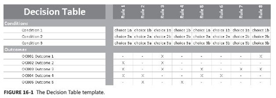
A Decision Table is represented as a grid, as shown in Figure 16-1. The top row contains labels for the business rules. The first column contains all the possible conditions and outcomes. Each of the remaining columns in the grid represents the outcomes valid for the specified choices. Collectively, the combination of choices and outcomes in a column make up each business rule.

A condition is an individual check such as “Lives in the United States - Yes or No” or “Marital status - single, married, divorced, or widowed.” We use the term “condition” instead of the more common term “decision” because “decision” implies that there is an order to the decision process, whereas “condition” does not.

The choices for a condition are the set of possible values for that condition. Choices can be binary, such as Yes or No or True or False; they can be multi-valued, such as ages 0-9, 10-21, 22-34, and 35+; or they can be a dash (-), meaning that the choice is irrelevant. The outcomes can have unique identifiers on them to help reference them from requirements.

Each outcome cell either contains an X, a number, a dash, or is left blank, as explained in Table 16-1.

A rule is the particular set of choices for each condition that have to match for the outcomes to apply. For example, the condition “lives in the United States = yes” and the condition “Marital status = single” could form the choices that make up a rule that says a specific outcome applies. The rules don’t have names; they are just permutations of all the possible choices of all the conditions and valid outcomes. Rules eventually become business rules in your requirements. For example, in the template, if the choices choice 1a, choice 2a, and choice 3a are true, then outcomes 2, 3, and 4 apply.

Example

An insurance company has a formalized process for determining which homeowner policies a customer is eligible for. Their decision process is modeled in the Decision Table in Figure 16-2. The model provides the assurance that all possible combinations are considered, because every combination of choice for every condition is included.

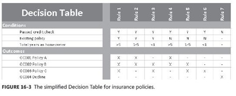
For example, the Decision Table tells us that if a customer has passed a credit check, has an existing policy, and has been a homeowner for 20 years, then he is eligible for policies A, B, and C. If the same customer did not have an existing policy, then he would be eligible for policies A and B.

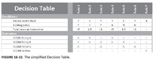
Looking at the complete table, you can see where unnecessary columns can be pruned. For example, being a homeowner and having existing policies with the company are irrelevant if the person fails the credit check. Figure 16-3 shows the simplified table.

Creating Decision Tables

The high-level steps for creating a Decision Table are outlined in Figure 16-4. We suggest an order to the steps; however, you might do this differently, as discussed later in this chapter, in the “Identify Outcomes” section. To illustrate how to create Decision Tables, this section continues with the example scenario from the previous section.

 

Identify Conditions

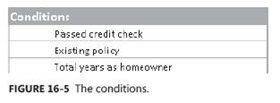
Think about all the potential conditions that apply to the situation and list them in the first column of your table. Conditions can be decisions that people make, data attributes that trigger various business rules, or any other factor (Gottesdiener 2005). Each condition needs its own row in the table. If you combined multiple conditions, it would be very hard to check for completeness. Figure 16-5 shows the first part of the table with just the possible conditions. A condition will often reference specific data fields from a Data Dictionary. In those cases, use the <object.field> notation, as described in Chapter 21, “Data Dictionary.”

Identify Choices

When you identify choices, you first need to determine what the choices are, then you might re-order your conditions in the table based on the choices, and then you enumerate the choices to build the rules columns.

Determining Valid Choices

After you have the conditions, consider the possible choices for each condition. Look at your Data Dictionary to identify valid values for the field. Some conditions will have binary choices of Yes and No or True and False, but the choices can be more complex, such as a range of numbers or matching words. There is no requirement that the conditions all be binary; in fact, the table can be simpler if a single multi-choice condition is used instead of several binary conditions. For example, if the condition is “Years as a homeowner,“ you might have three potential choices for that condition that should be modeled: more than five years, one to five years, and less than one year.

Make sure that the choices you use reflect all possible choices for the condition. If you miss any possible choices, your table will be incomplete and you cannot guarantee that you have all of the requirements. For a particular condition, the choices must also be mutually exclusive, in that only one can exist at a time. A condition cannot have overlapping ranges such that each could simultaneously match because they share values. For example, the ranges 0–1 and 1–5 overlap because each includes the number 1. If you need to specify ranges like this, use the following type of range definitions instead: <1 and 1–5, or <=1 and >1–5.

Reordering Conditions

You do not need to list the conditions in any specific order; however, it is generally easier to make a table when they are listed in the order of number of choices. The condition that has the fewest choices should be the first condition. For example, if you have a rule such as, “If the customer failed the credit check, then automatically decline him,“ then you can cut out half of your permutations. You don’t need to do any work to evaluate the rest of the conditions; they just don’t matter. The condition that has the most choices should be the last condition listed. This order puts the most constraining conditions at the top of the list, which aids you in reviewing and simplifying the table.

Enumerating Choices

Now you add rules (columns) to enumerate all possible combinations of choices for all conditions. If you multiply the number of choices together for each condition, you can determine how many columns you need. If you have just one condition with two choices, you will need only two columns. If you have three conditions with two choices each, you will need eight columns (2 x 2 x 2 = 8). In this example, there are two choices for the first condition (Y or N), two for the second condition (Y or N), and three for the third condition (>5, 1–5, or<1), so there are 12 columns (2 x 2 x 3 = 12).

In addition to each choice being mutually exclusive, each rule needs to be mutually exclusive. This means that you should have no columns with the same set of choices.

The order of the rules should make it easy to recognize that all possible choices of conditions are being examined. In the first row, group all the like choices together. In the example, for the first condition, half will be Y and half will be N, so make the first four columns Y and the second four N, as in Figure 16-6.

For the second condition, half of the Ys from the first condition will be Y and half will be N. This results in the pattern in Figure 16-7.

Finally, in the third condition, alternate the three choices again to get the pattern in Figure 16-8. When you complete the conditions and choices of a Decision Table, you will get a result that looks like this. Remember that you will have more columns if you have more conditions or valid choices for conditions.

Identify Outcomes

The combinations of choices lead to one or more outcomes. Outcomes are the decisions, conclusions, or actions that occur when the choices are valid. Add the outcomes to the first column of your table, below all of the conditions. Figure 16-9 shows our same scenario with outcomes added.

You might find it easier to identify the outcomes first. If you know your outcomes and want to determine the conditions under which they are valid, start with the outcomes part of the table and then identify conditions and choices. It is possible that you might start with a few business rules, so creating the table with just a few rules filled in can quickly show where there are gaps in your information.

Label Valid Outcomes by Choice Combinations

Each column now represents a possible combination of choices for the conditions. Label the valid outcomes under the combination of choices. If you know that an outcome is not valid, mark it with a dash, and if you are not sure, leave it blank to follow up later. Figure 16-10 shows the resulting Decision Table for the scenario.

Simplify the Decision Table

Because so many columns are necessary even with just a few conditions, it is best to try to simplify your table as early in the process as feasible. If there are specific rules that are only dependent on a few of the conditions, that means that you do not need to evaluate other conditions. You should combine the rules to remove the ones that differ in conditions and not in outcomes.

When a condition is irrelevant to the outcome, put a dash in the cell for that condition. Do not just haphazardly delete columns, though! You must ensure that all combinations are included in the table, using the dash to represent those conditions whose choices do not matter. For example, you know that when a customer fails the credit check, she is declined, so you do not need to evaluate the existing-policy or years-as-a-homeowner conditions. Figure 16-11 shows the example after it has been simplified.

In simplifying your table, you might discover that some conditions are always irrelevant. You can remove those conditions and further condense your table. Finally, if, after you complete your table, you see that certain outcomes are always executed in tandem, you can combine those outcomes into a single outcome.