
Computer-aided engineering services on Azure
Provide a software-as-a-service (SaaS) platform for computer-aided engineering (CAE) on Azure.
This browser is no longer supported.
Upgrade to Microsoft Edge to take advantage of the latest features, security updates, and technical support.
High-performance computing (HPC), also called "big compute", uses a large number of CPU or GPU-based computers to solve complex mathematical tasks.
Many industries use HPC to solve some of their most difficult problems. These include workloads such as:
One of the primary differences between an on-premises HPC system and one in the cloud is the ability for resources to dynamically be added and removed as they're needed. Dynamic scaling removes compute capacity as a bottleneck and instead allow customers to right size their infrastructure for the requirements of their jobs.
The following articles provide more detail about this dynamic scaling capability.
As you're looking to implement your own HPC solution on Azure, ensure you're reviewed the following topics:
There are many infrastructure components that are necessary to build an HPC system. Compute, storage, and networking provide the underlying components, no matter how you choose to manage your HPC workloads.
There are many different ways to design and implement your HPC architecture on Azure. HPC applications can scale to thousands of compute cores, extend on-premises clusters, or run as a 100% cloud-native solution.
The following scenarios outline a few of the common ways HPC solutions are built.
Provide a software-as-a-service (SaaS) platform for computer-aided engineering (CAE) on Azure.

Run native HPC workloads in Azure using the Azure Batch service
Azure offers a range of sizes that are optimized for both CPU & GPU intensive workloads.
N-series VMs feature NVIDIA GPUs designed for compute-intensive or graphics-intensive applications including artificial intelligence (AI) learning and visualization.
Large-scale Batch and HPC workloads have demands for data storage and access that exceed the capabilities of traditional cloud file systems. There are many solutions that manage both the speed and capacity needs of HPC applications on Azure:
For more information comparing Lustre, GlusterFS, and BeeGFS on Azure, review the Parallel Files Systems on Azure e-book and the Lustre on Azure blog.
H16r, H16mr, A8, and A9 VMs can connect to a high throughput back-end RDMA network. This network can improve the performance of tightly coupled parallel applications running under Microsoft Message Passing Interface better known as MPI or Intel MPI.
Building an HPC system from scratch on Azure offers a significant amount of flexibility, but it is often very maintenance intensive.
If you have an existing on-premises HPC system that you'd like to connect to Azure, there are several resources to help get you started.
First, review the Options for connecting an on-premises network to Azure article in the documentation. From there, you can find additional information on these connectivity options:
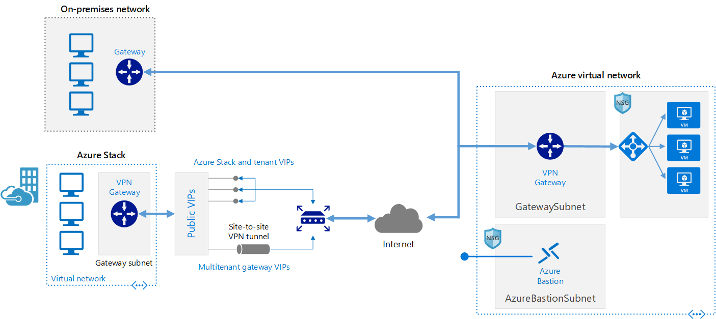
This reference architecture shows how to extend an on-premises network to Azure, using a site-to-site virtual private network (VPN).
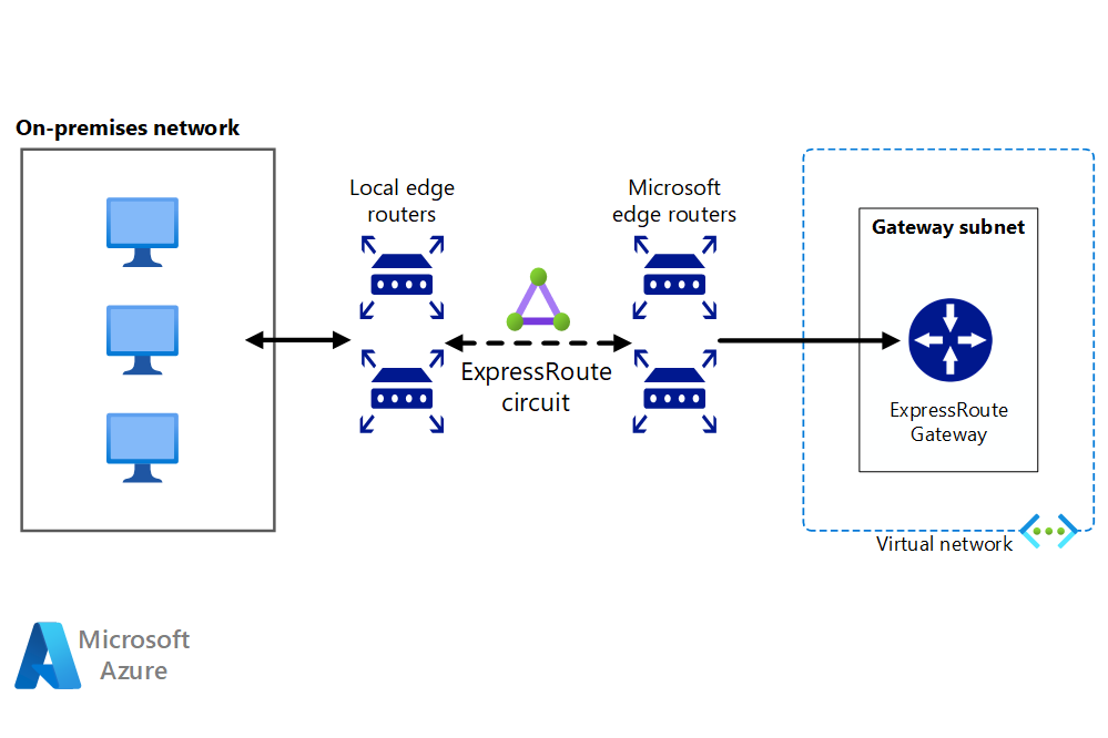
ExpressRoute connections use a private, dedicated connection through a third-party connectivity provider. The private connection extends your on-premises network into Azure.
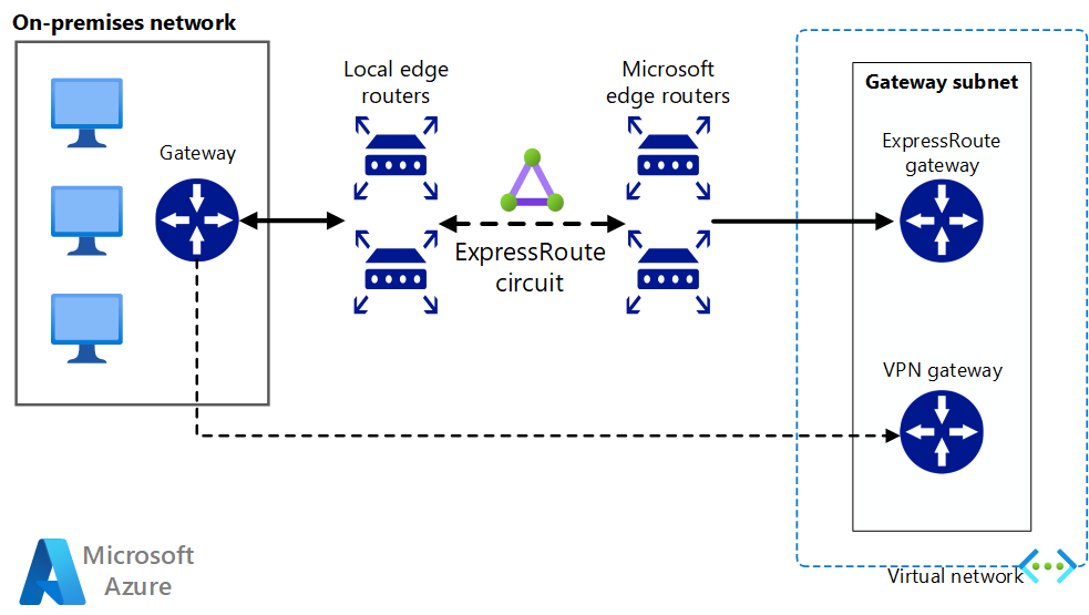
Implement a highly available and secure site-to-site network architecture that spans an Azure virtual network and an on-premises network connected using ExpressRoute with VPN gateway failover.
Once network connectivity is securely established, you can start using cloud compute resources on-demand with the bursting capabilities of your existing workload manager.
There are many workload managers offered in the Azure Marketplace.
Azure Batch is a platform service for running large-scale parallel and HPC applications efficiently in the cloud. Azure Batch schedules compute-intensive work to run on a managed pool of virtual machines, and can automatically scale compute resources to meet the needs of your jobs.
SaaS providers or developers can use the Batch SDKs and tools to integrate HPC applications or container workloads with Azure, stage data to Azure, and build job execution pipelines.
In Azure Batch all the services are running on the Cloud, the image below shows how the architecture looks with Azure Batch, having the scalability and job schedule configurations running in the Cloud while the results and reports can be sent to your on-premises environment.

Azure CycleCloud Provides the simplest way to manage HPC workloads using any scheduler (like Slurm, Grid Engine, HPC Pack, HTCondor, LSF, PBS Pro, or Symphony), on Azure
CycleCloud allows you to:
In this Hybrid example diagram, we can see clearly how these services are distributed between the cloud and the on-premises environment. Having the opportunity to run jobs in both workloads.

The cloud native model example diagram below, shows how the workload in the cloud will handle everything while still conserving the connection to the on-premises environment.

| Feature | Azure Batch | Azure CycleCloud |
|---|---|---|
| Scheduler | Batch APIs and tools and command-line scripts in the Azure portal (Cloud Native). | Use standard HPC schedulers such as Slurm, PBS Pro, LSF, Grid Engine, and HTCondor, or extend CycleCloud autoscaling plugins to work with your own scheduler. |
| Compute Resources | Software as a Service Nodes – Platform as a Service | Platform as a Service Software – Platform as a Service |
| Monitor Tools | Azure Monitor | Azure Monitor, Grafana |
| Customization | Custom image pools, Third Party images, Batch API access. | Use the comprehensive RESTful API to customize and extend functionality, deploy your own scheduler, and support into existing workload managers |
| Integration | Synapse Pipelines, Azure Data Factory, Azure CLI | Built-In CLI for Windows and Linux |
| User type | Developers | Classic HPC administrators and users |
| Work Type | Batch, Workflows | Tightly coupled (Message Passing Interface/MPI). |
| Windows Support | Yes | Varies, depending on scheduler choice |
The following are examples of cluster and workload managers that can run in Azure infrastructure. Create stand-alone clusters in Azure VMs or burst to Azure VMs from an on-premises cluster.
Containers can also be used to manage some HPC workloads. Services like the Azure Kubernetes Service (AKS) makes it simple to deploy a managed Kubernetes cluster in Azure.
Managing your HPC cost on Azure can be done through a few different ways. Ensure you've reviewed the Azure purchasing options to find the method that works best for your organization.
For an overview of security best practices on Azure, review the Azure Security Documentation.
In addition to the network configurations available in the Cloud Bursting section, you can implement a hub/spoke configuration to isolate your compute resources:

The hub is a virtual network (VNet) in Azure that acts as a central point of connectivity to your on-premises network. The spokes are VNets that peer with the hub, and can be used to isolate workloads.
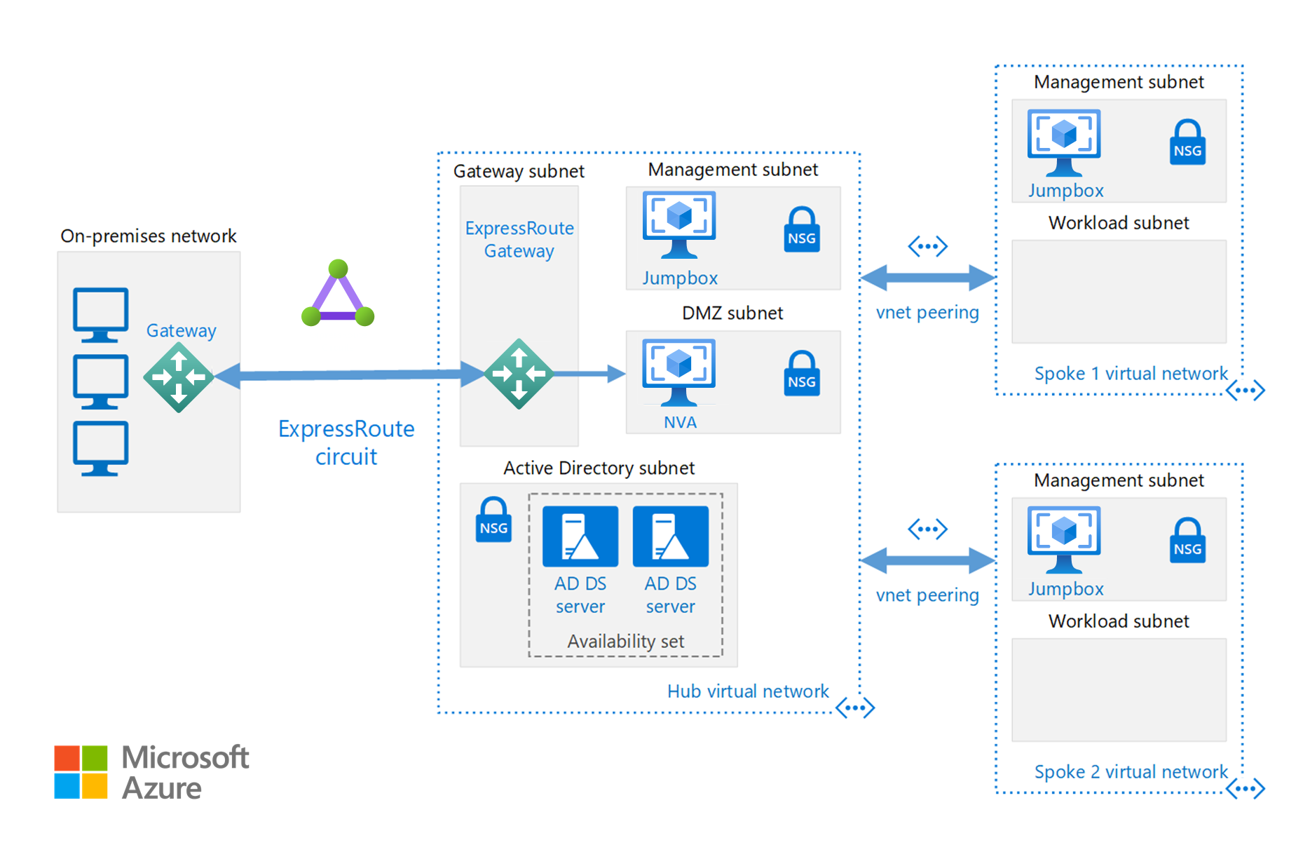
This reference architecture builds on the hub-spoke reference architecture to include shared services in the hub that can be consumed by all spokes.
Run custom or commercial HPC applications in Azure. Several examples in this section are benchmarked to scale efficiently with additional VMs or compute cores. Visit the Azure Marketplace for ready-to-deploy solutions.
Note
Check with the vendor of any commercial application for licensing or other restrictions for running in the cloud. Not all vendors offer pay-as-you-go licensing. You might need a licensing server in the cloud for your solution, or connect to an on-premises license server.
Run GPU-powered virtual machines in Azure in the same region as the HPC output for the lowest latency, access, and to visualize remotely through Azure Virtual Desktop.
There are many customers who have seen great success by using Azure for their HPC workloads. You can find a few of these customer case studies below:
For the latest announcements, see the following resources:
These tutorials will provide you with details on running applications on Microsoft Batch:
