Note
Access to this page requires authorization. You can try signing in or changing directories.
Access to this page requires authorization. You can try changing directories.
Azure Cosmos DB is a schema-agnostic database that allows you to iterate on your application without having to deal with schema or index management. By default, Azure Cosmos DB automatically indexes every property for all items in your container without having to define any schema or configure secondary indexes.
This article explains how Azure Cosmos DB indexes data and how it uses indexes to improve query performance. It's recommended to go through this section before exploring how to customize indexing policies.
From items to trees
Every time an item is stored in a container, its content is projected as a JSON document, then converted into a tree representation. This conversion means that every property of that item gets represented as a node in a tree. A pseudo root node is created as a parent to all the first-level properties of the item. The leaf nodes contain the actual scalar values carried by an item.
As an example, consider this item:
{
  "locations": [
    { "country": "Germany", "city": "Berlin" },
    { "country": "France", "city": "Paris" }
  ],
  "headquarters": { "country": "Belgium", "employees": 250 },
  "exports": [
    { "city": "Moscow" },
    { "city": "Athens" }
  ]
}
This tree represents the example JSON item:
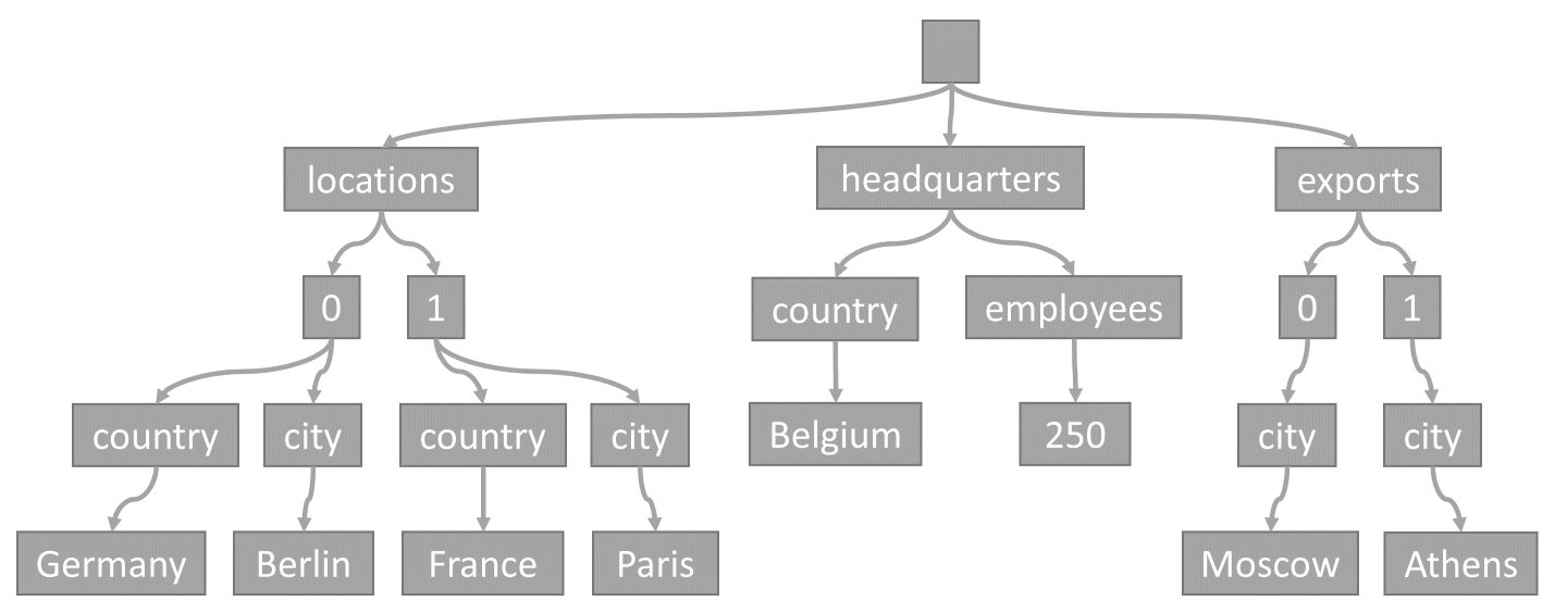
Note how arrays are encoded in the tree: every entry in an array gets an intermediate node labeled with the index of that entry within the array (0, 1 etc.).
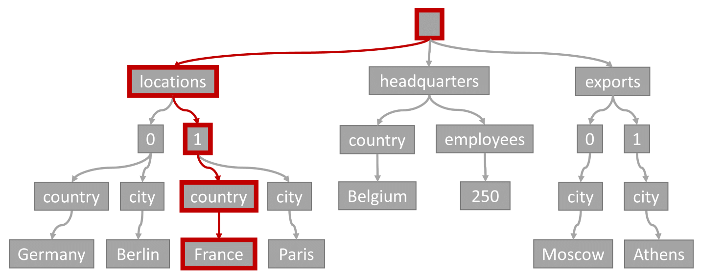
From trees to property paths
Azure Cosmos DB transforms items into trees because it allows the system to reference properties using their paths within those trees. To get the path for a property, we can traverse the tree from the root node to that property, and concatenate the labels of each traversed node.
Here are the paths for each property from the example item described previously:
/locations/0/country: "Germany"/locations/0/city: "Berlin"/locations/1/country: "France"/locations/1/city: "Paris"/headquarters/country: "Belgium"/headquarters/employees: 250/exports/0/city: "Moscow"/exports/1/city: "Athens"
Azure Cosmos DB effectively indexes each property's path and its corresponding value when an item is written.
Index types
Azure Cosmos DB currently supports three types of indexes. You can configure these index types when defining the indexing policy.
Range index
Range indexes are based on an ordered tree-like structure. The range index type is used for:
Equality queries:
SELECT * FROM container c WHERE c.property = 'value'SELECT * FROM c WHERE c.property IN ("value1", "value2", "value3")Equality match on an array element
SELECT * FROM c WHERE ARRAY_CONTAINS(c.tags, "tag1")Range queries:
SELECT * FROM container c WHERE c.property > 'value'Note
Works for
>,<,>=,<=,!=Checking for the presence of a property:
SELECT * FROM c WHERE IS_DEFINED(c.property)String system functions:
SELECT * FROM c WHERE CONTAINS(c.property, "value")SELECT * FROM c WHERE STRINGEQUALS(c.property, "value")ORDER BYqueries:SELECT * FROM container c ORDER BY c.propertyJOINqueries:SELECT child FROM container c JOIN child IN c.properties WHERE child = 'value'
Range indexes can be used on scalar values (string or number). The default indexing policy for newly created containers enforces range indexes for any string or number. To learn how to configure range indexes, see Manage indexing policies in Azure Cosmos DB.
Note
An ORDER BY clause that orders by a single property always needs a range index and fails if the path it references doesn't have one. Similarly, an ORDER BY query that orders by multiple properties always needs a composite index.
Spatial index
Spatial indexes enable efficient queries on geospatial objects such as points, lines, polygons, and multipolygons. These queries use ST_DISTANCE, ST_WITHIN, ST_INTERSECTS keywords. The following are some examples that use spatial index type:
Geospatial distance queries:
SELECT * FROM container c WHERE ST_DISTANCE(c.property, { "type": "Point", "coordinates": [0.0, 10.0] }) < 40Geospatial within queries:
SELECT * FROM container c WHERE ST_WITHIN(c.property, {"type": "Point", "coordinates": [0.0, 10.0] })Geospatial intersect queries:
SELECT * FROM c WHERE ST_INTERSECTS(c.property, { 'type':'Polygon', 'coordinates': [[ [31.8, -5], [32, -5], [31.8, -5] ]] })
Spatial indexes can be used on correctly formatted GeoJSON objects. Points, LineStrings, Polygons, and MultiPolygons are currently supported. To learn how to configure spatial indexes, see Manage indexing policies in Azure Cosmos DB.
Composite indexes
Composite indexes increase the efficiency when you're performing operations on multiple fields. The composite index type is used for:
ORDER BYqueries on multiple properties:SELECT * FROM container c ORDER BY c.property1, c.property2Queries with a filter and
ORDER BY. These queries can utilize a composite index if the filter property is added to theORDER BYclause.SELECT * FROM container c WHERE c.property1 = 'value' ORDER BY c.property1, c.property2Queries with a filter on two or more properties where at least one property is an equality filter:
SELECT * FROM container c WHERE c.property1 = 'value' AND c.property2 > 'value'
As long as one filter predicate uses one of the index types, the query engine evaluates that first before scanning the rest. For example, if you have a SQL query such as SELECT * FROM c WHERE c.firstName = "Andrew" and CONTAINS(c.lastName, "Liu"):
This query first filters for entries where firstName = "Andrew" by using the index. It then passes all of the firstName = "Andrew" entries through a subsequent pipeline to evaluate the CONTAINS filter predicate.
You can speed up queries and avoid full container scans when using functions that perform a full scan like CONTAINS. You can add more filter predicates that use the index to speed up these queries. The order of filter clauses isn't important. The query engine figures out which predicates are more selective and run the query accordingly.
To learn how to configure composite indexes, see Manage indexing policies in Azure Cosmos DB.
Vector indexes
Vector indexes increase the efficiency when performing vector searches using the VectorDistance system function. Vector searches have significantly lower latency, higher throughput, and less RU consumption when using a vector index. Azure Cosmos DB for NoSQL supports any vector embeddings (text, image, multimodal, etc.) under 4,096 dimensions in size.
To learn how to configure vector indexes, see Vector indexing policy examples.
ORDER BYvector search queries:SELECT TOP 10 * FROM c ORDER BY VectorDistance(c.vector1, c.vector2)Projection of the similarity score in vector search queries:
SELECT TOP 10 c.name, VectorDistance(c.vector1, c.vector2) AS SimilarityScore
FROM c
ORDER BY VectorDistance(c.vector1, c.vector2)
Range filters on the similarity score.
SELECT TOP 10 *
FROM c
WHERE VectorDistance(c.vector1, c.vector2) > 0.8
ORDER BY VectorDistance(c.vector1, c.vector2)
Important
Currently, vector policies and vector indexes are immutable after creation. To make changes, create a new collection.
Index usage
There are five ways that the query engine can evaluate query filters, sorted by most-efficient to least-efficient:
- Index seek
- Precise index scan
- Expanded index scan
- Full index scan
- Full scan
When you index property paths, the query engine automatically uses the index as efficiently as possible. Aside from indexing new property paths, you don't need to configure anything to optimize how queries use the index. A query's RU charge is a combination of both the RU charge from index usage and the RU charge from loading items.
The following table summarizes the different ways indexes are used in Azure Cosmos DB:
| Index lookup type | Description | Common examples | RU charge from index usage | RU charges from loading items from transactional data store |
|---|---|---|---|---|
| Index seek | Read only required indexed values and load only matching items from the transactional data store | Equality filters, IN | Constant per equality filter | Increases based on number of items in query results |
| Precise index scan | Binary search of indexed values and load only matching items from the transactional data store | Range comparisons (>, <, <=, or >=), StartsWith | Comparable to index seek, increases slightly based on the cardinality of indexed properties | Increases based on number of items in query results |
| Expanded index scan | Optimized search (but less efficient than a binary search) of indexed values and load only matching items from the transactional data store | StartsWith (case-insensitive), StringEquals (case-insensitive) | Increases slightly based on the cardinality of indexed properties | Increases based on number of items in query results |
| Full index scan | Read distinct set of indexed values and load only matching items from the transactional data store | Contains, EndsWith, RegexMatch, LIKE | Increases linearly based on the cardinality of indexed properties | Increases based on number of items in query results |
| Full scan | Load all items from the transactional data store | Upper, Lower | N/A | Increases based on number of items in container |
When writing queries, you should use filter predicates that use the index as efficiently as possible. For example, if either StartsWith or Contains would work for your use case, you should opt for StartsWith since it does a precise index scan instead of a full index scan.
Index usage details
This section covers more details about how queries use indexes. This level of detail isn't necessary to learn how to get started with Azure Cosmos DB but is documented in detail for curious users. We reference the example item shared earlier in this document:
Example items:
{
  "id": 1,
  "locations": [
    { "country": "Germany", "city": "Berlin" },
    { "country": "France", "city": "Paris" }
  ],
  "headquarters": { "country": "Belgium", "employees": 250 },
  "exports": [
    { "city": "Moscow" },
    { "city": "Athens" }
  ]
}
{
  "id": 2,
  "locations": [
    { "country": "Ireland", "city": "Dublin" }
  ],
  "headquarters": { "country": "Belgium", "employees": 200 },
  "exports": [
    { "city": "Moscow" },
    { "city": "Athens" },
    { "city": "London" }
  ]
}
Azure Cosmos DB uses an inverted index. The index works by mapping each JSON path to the set of items that contain that value. The item ID mapping is represented across many different index pages for the container. Here's a sample diagram of an inverted index for a container that includes the two example items:
| Path | Value | List of item IDs |
|---|---|---|
| /locations/0/country | Germany | 1 |
| /locations/0/country | Ireland | 2 |
| /locations/0/city | Berlin | 1 |
| /locations/0/city | Dublin | 2 |
| /locations/1/country | France | 1 |
| /locations/1/city | Paris | 1 |
| /headquarters/country | Belgium | 1, 2 |
| /headquarters/employees | 200 | 2 |
| /headquarters/employees | 250 | 1 |
The inverted index has two important attributes:
- For a given path, values are sorted in ascending order. Therefore, the query engine can easily serve
ORDER BYfrom the index. - For a given path, the query engine can scan through the distinct set of possible values to identify the index pages where there are results.
The query engine can utilize the inverted index in four different ways:
Index seek
Consider the following query:
SELECT location
FROM location IN company.locations
WHERE location.country = 'France'
The query predicate (filtering on items where any location has "France" as its country or region) would match the path highlighted in this diagram:
Since this query has an equality filter, after traversing this tree, we can quickly identify the index pages that contain the query results. In this case, the query engine would read index pages that contain Item 1. An index seek is the most efficient way to use the index. With an index seek, we only read the necessary index pages and load only the items in the query results. Therefore, the index lookup time and RU charge from index lookup are incredibly low, regardless of the total data volume.
Precise index scan
Consider the following query:
SELECT *
FROM company
WHERE company.headquarters.employees > 200
The query predicate (filtering on items where there are more than 200 employees) can be evaluated with a precise index scan of the headquarters/employees path. When doing a precise index scan, the query engine starts by doing a binary search of the distinct set of possible values to find the location of the value 200 for the headquarters/employees path. Since the values for each path are sorted in ascending order, it's easy for the query engine to do a binary search. After the query engine finds the value 200, it starts reading all remaining index pages (going in the ascending direction).
Because the query engine can do a binary search to avoid scanning unnecessary index pages, precise index scans tend to have comparable latency and RU charges to index seek operations.
Expanded index scan
Consider the following query:
SELECT *
FROM company
WHERE STARTSWITH(company.headquarters.country, "United", true)
The query predicate (filtering on items that have headquarters in a location that starts with case-insensitive "United") can be evaluated with an expanded index scan of the headquarters/country path. Operations that do an expanded index scan have optimizations that can help avoid needs to scan every index page but are slightly more expensive than a precise index scan's binary search.
For example, when evaluating case-insensitive StartsWith, the query engine checks the index for different possible combinations of uppercase and lowercase values. This optimization allows the query engine to avoid reading most index pages. Different system functions have different optimizations that they can use to avoid reading every index page, so they're broadly categorized as expanded index scan.
Full index scan
Consider the following query:
SELECT *
FROM company
WHERE CONTAINS(company.headquarters.country, "United")
The query predicate (filtering on items that have headquarters in a location that contains "United") can be evaluated with an index scan of the headquarters/country path. Unlike a precise index scan, a full index scan always scans through the distinct set of possible values to identify the index pages where there are results. In this case, CONTAINS is run on the index. The index lookup time and RU charge for index scans increases as the cardinality of the path increases. In other words, the more possible distinct values that the query engine needs to scan, the higher the latency and RU charge involved in doing a full index scan.
For example, consider two properties: town and country. The cardinality of town is 5,000 and the cardinality of country is 200. Here are two example queries that each have a CONTAINS system function that does a full index scan on the town property. The first query uses more RUs than the second query because the cardinality of town is higher than country.
SELECT *
FROM c
WHERE CONTAINS(c.town, "Red", false)
SELECT *
FROM c
WHERE CONTAINS(c.country, "States", false)
Full scan
In some cases, the query engine might not be able to evaluate a query filter using the index. In this case, the query engine needs to load all items from the transactional store in order to evaluate the query filter. Full scans don't use the index and have an RU charge that increases linearly with the total data size. Luckily, operations that require full scans are rare.
Vector search queries without a defined vector index
If you don't define a vector index policy and use the VectorDistance system function in an ORDER BY clause, then this results in a full scan and have an RU charge higher than if you defined a vector index policy. Similarity, if you use VectorDistance with the brute force boolean value set to true, and don't have a flat index defined for the vector path, then a full scan occurs.
Queries with complex filter expressions
In the earlier examples, we only considered queries that had simple filter expressions (for example, queries with just a single equality or range filter). In reality, most queries have much more complex filter expressions.
Consider the following query:
SELECT *
FROM company
WHERE company.headquarters.employees = 200 AND CONTAINS(company.headquarters.country, "United")
To execute this query, the query engine must do an index seek on headquarters/employees and full index scan on headquarters/country. The query engine has internal heuristics that it uses to evaluate the query filter expression as efficiently as possible. In this case, the query engine would avoid needing to read unnecessary index pages by doing the index seek first. If for example, only 50 items matched the equality filter, the query engine would only need to evaluate CONTAINS on the index pages that contained those 50 items. A full index scan of the entire container wouldn't be necessary.
Index utilization for scalar aggregate functions
Queries with aggregate functions must rely exclusively on the index in order to use it.
In some cases, the index can return false positives. For example, when evaluating CONTAINS on the index, the number of matches in the index might exceed the number of query results. The query engine loads all index matches, evaluates the filter on the loaded items, and returns only the correct results.
For most queries, loading false positive index matches doesn't have any noticeable effect on index utilization.
For example, consider the following query:
SELECT *
FROM company
WHERE CONTAINS(company.headquarters.country, "United")
The CONTAINS system function might return some false positive matches, so the query engine needs to verify whether each loaded item matches the filter expression. In this example, the query engine might only need to load an extra few items, so the effect on index utilization and RU charge is minimal.
However, queries with aggregate functions must rely exclusively on the index in order to use it. For example, consider the following query with a COUNT aggregate:
SELECT COUNT(1)
FROM company
WHERE CONTAINS(company.headquarters.country, "United")
Like in the first example, the CONTAINS system function might return some false positive matches. Unlike the SELECT * query, however, the COUNT query can't evaluate the filter expression on the loaded items to verify all index matches. The COUNT query must rely exclusively on the index, so if there's a chance a filter expression returns false positive matches, the query engine resorts to a full scan.
Queries with the following aggregate functions must rely exclusively on the index, so evaluating some system functions requires a full scan.