Declarative feature engineering and managed pipelines

Important

This feature is Beta and is available in the following regions: us-east-1 and us-west-2.

The feature store declarative APIs enable you to define and compute time-windowed aggregation features from data sources. This guide covers the following workflows:

Feature development workflow
- Use create_feature to define Unity Catalog feature objects that can be used in model training and serving workflows.
Model training workflow
- Use create_training_set to calculate point-in-time aggregated features for machine learning. This will return a training set object that can return a Spark DataFrame with computed features augmented to the observation dataset for training a model.
- Calling log_model with this training set, to save this model in Unity Catalog, along with lineage between feature and model objects.
- score_batch uses Unity Catalog lineage to use feature definition code to perform point-in-time correct feature aggregations augmented to the inference dataset for model scoring.
Feature materialization and serving workflow
- After defining a feature with create_feature or retrieving it using get_feature, you can use materialize_features to materialize the feature or set of features to an offline store for efficient reuse, or to an online store for online serving.
- Use create_training_set with the materialized view to prepare an offline batch training dataset.

For detailed documentation on log_model and score_batch, see Use features to train models.

Requirements

A classic compute cluster running Databricks Runtime 17.0 ML or above.
You must install the custom Python package. The following lines of code must be executed each time a notebook is run:
```
%pip install databricks-feature-engineering>=0.14.0
dbutils.library.restartPython()
```

Quickstart example

from databricks.feature_engineering import FeatureEngineeringClient
from databricks.feature_engineering.entities import DeltaTableSource, Sum, Avg, ContinuousWindow, OfflineStoreConfig
from datetime import timedelta

CATALOG_NAME = "main"
SCHEMA_NAME = "feature_store"
TABLE_NAME = "transactions"

# 1. Create data source
source = DeltaTableSource(
    catalog_name=CATALOG_NAME,
    schema_name=SCHEMA_NAME,
    table_name=TABLE_NAME,
    entity_columns=["user_id"],
    timeseries_column="transaction_time"
)

# 2. Define features
fe = FeatureEngineeringClient()
features = [
    fe.create_feature(
        catalog_name=CATALOG_NAME,
        schema_name=SCHEMA_NAME,
        name="avg_transaction_30d",
        source=source,
        inputs=["amount"],
        function=Avg(),
        time_window=ContinuousWindow(window_duration=timedelta(days=30))
    ),
    fe.create_feature(
        catalog_name=CATALOG_NAME,
        schema_name=SCHEMA_NAME,
        source=source,
        inputs=["amount"],
        function=Sum(),
        time_window=ContinuousWindow(window_duration=timedelta(days=7))
        # name auto-generated: "amount_sum_continuous_7d"
    ),
]

# 3. Create training set using declarative features

`labeled_df` should have columns "user_id", "transaction_time", and "target". It can have other context features specific to the individual observations.
training_set = fe.create_training_set(
    df=labeled_df,
    features=features,
    label="target",
)
training_set.load_df().display()  # action: joins labeled_df with computed feature

# 4. Train model
with mlflow.start_run():
    training_df = training_set.load_df()

    # training code

    fe.log_model(
        model=model,
        artifact_path="recommendation_model",
        flavor=mlflow.sklearn,
        training_set=training_set,
        registered_model_name=f"{CATALOG_NAME}.{SCHEMA_NAME}.recommendation_model",
    )

# 5. (Optional) Materialize features for serving
fe.materialize_features(
    features=features,
    offline_config=OfflineStoreConfig(
        catalog_name=CATALOG_NAME,
        schema_name=SCHEMA_NAME,
        table_name_prefix="customer_features"
    ),
    pipeline_state="ACTIVE",
    cron_schedule="0 0 * * * ?"  # Hourly
)

Note

After materializing features, you can serve models using CPU model serving. For details on online serving, see Materialize and serve declarative features.

Data sources

`DeltaTableSource`

Note

Permitted data types for timeseries_column: TimestampType, DateType. Other integer data types can work but will cause loss in precision for time window aggregates.

The following code shows an example using the main.analytics.user_events table from Unity Catalog:

from databricks.feature_engineering.entities import DeltaTableSource

source = DeltaTableSource(
    catalog_name="main",               # Catalog name
    schema_name="analytics",           # Schema name
    table_name="user_events",          # Table name
    entity_columns=["user_id"],        # Join keys, used to look up features for an entity
    timeseries_column="event_time"     # Timestamp for time windows
)

Declarative feature API

`create_feature()` API

FeatureEngineeringClient.create_feature() provides comprehensive validation and ensures proper feature construction:

FeatureEngineeringClient.create_feature(
    source: DataSource,                   # Required: DeltaTableSource
    inputs: List[str],                    # Required: List of column names from the source
    function: Union[Function, str],       # Required: Aggregation function (Sum, Avg, Count, etc.)
    time_window: TimeWindow,              # Required: TimeWindow for aggregation
    catalog_name: str,                    # Required: The catalog name for the feature
    schema_name: str,                     # Required: The schema name for the feature
    name: Optional[str],                  # Optional: Feature name (auto-generated if omitted)
    description: Optional[str],           # Optional: Feature description
    filter_condition: Optional[str],      # Optional: SQL WHERE clause to filter source data
) -> Feature

Parameters:

source: The data source used in feature computation
inputs: List of column names from the source to use as input for aggregation
function: The aggregation function (Function instance or string name). See list of supported functions below.
time_window: The time window for aggregation (TimeWindow instance or dict with 'duration' and optional 'offset')
catalog_name: The catalog name for the feature
schema_name: The schema name for the feature
name: Optional feature name (auto-generated if omitted)
description: Optional description of the feature
filter_condition: Optional SQL WHERE clause to filter source data before aggregation. Example: "status = 'completed'", "transaction" = "Credit" AND "amount > 100"

Returns: A validated Feature instance

Raises: ValueError if any validation fails

Auto-generated names

When name is omitted, names follow the pattern: {column}_{function}_{window}. For example:

price_avg_continuous_1h (1-hour average price)
transaction_count_continuous_30d_1d (30-day count of transaction with 1d offset from event timestamp)

Supported functions

Note

All functions are applied over an aggregation time-window as described in the time windows section below.

Function	Shorthand	Description	Example use case
`Sum()`	`"sum"`	Total of values	Per user daily app usage in minutes
`Avg()`	`"avg"`, `"mean"`	Average of values	Mean transaction amount
`Count()`	`"count"`	Number of records	Number of logins per user
`Min()`	`"min"`	Minimum value	Lowest heart rate recorded by a wearable device
`Max()`	`"max"`	Maximum value	Maximum basket size of times per session
`StddevPop()`	`"stddev_pop"`	Population standard deviation	Daily transaction amount variability across all customers
`StddevSamp()`	`"stddev_samp"`	Sample standard deviation	Variability of ad campaign click-through rates
`VarPop()`	`"var_pop"`	Population variance	Spread of sensor readings for IoT devices in a factory
`VarSamp()`	`"var_samp"`	Sample variance	Spread of movie ratings over a sampled group
`ApproxCountDistinct(relativeSD=0.05)`	`"approx_count_distinct"`*	Approximate unique count	Distinct count of items purchased
`ApproxPercentile(percentile=0.95,accuracy=100)`	N/A	Approximate percentile	p95 response latency
`First()`	`"first"`	First value	First login timestamp
`Last()`	`"last"`	Last value	Most recent purchase amount

*Functions with parameters use default values when using string shorthand.

The following example shows window-aggregation features defined over the same data source.

from databricks.feature_engineering.entities import Sum, Avg, Count, Max, ApproxCountDistinct

fe = FeatureEngineeringClient()
sum_feature = fe.create_feature(source=source, inputs=["amount"], function=Sum(), ...)
avg_feature = fe.create_feature(source=source, inputs=["amount"], function=Avg(), ...)
distinct_count = fe.create_feature(
    source=source,
    inputs=["product_id"],
    function=ApproxCountDistinct(relativeSD=0.01),
    ...
)

Features with filter conditions

The declarative feature APIs also support applying a SQL filter, which is applied as a WHERE clause in aggregations. Filters are useful when working with large source tables that include a superset of data needed for feature computation, and minimizes the need for creating separate views on top of these tables.

from databricks.feature_engineering.entities import Sum, Count, ContinuousWindow
from datetime import timedelta

# Only aggregate high-value transactions
high_value_sales = fe.create_feature(
    catalog_name="main",
    schema_name="ecommerce",
    source=transactions,
    inputs=["amount"],
    function=Sum(),
    time_window=ContinuousWindow(window_duration=timedelta(days=30)),
    filter_condition="amount > 100"  # Only transactions over $100
)

# Multiple conditions using SQL syntax
completed_orders = fe.create_feature(
    catalog_name="main",
    schema_name="ecommerce",
    source=orders,
    inputs=["order_id"],
    function=Count(),
    time_window=ContinuousWindow(window_duration=timedelta(days=7)),
    filter_condition="status = 'completed' AND payment_method = 'credit_card'"
)

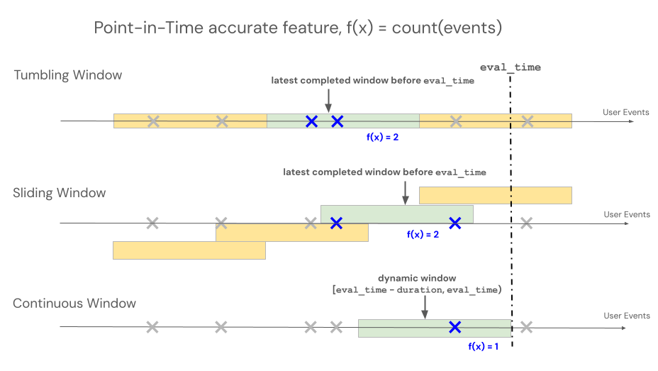
Time windows

Feature engineering declarative APIs support three different window types to control lookback behavior for time window-based aggregations: continuous, tumbling, and sliding.

Continuous windows look back from the event time. Duration and offset are explicitly defined.
Tumbling windows are fixed, non-overlapping time windows. Each data point belongs to exactly one window.
Sliding windows are overlapping, rolling time windows with a configurable slide interval.

The following illustration shows how they work.

Continuous, tumbling, and sliding lookback windows.

Continuous window

Continuous windows are up-to-date and real-time aggregates, typically used over streaming data. In streaming pipelines, the continuous window emits a new row only when the contents of the fixed-length window change, such as when an event enters or leaves. When a continuous window feature is used in training pipelines, an accurate point-in-time feature calculation is performed on the source data using the fixed-length window duration immediately preceding a specific event's timestamp. This helps prevent online-offline skew or data leakage. Features at time T aggregate events from [T − duration, T).

class ContinuousWindow(TimeWindow):
    window_duration: datetime.timedelta
    offset: Optional[datetime.timedelta] = None

The following table lists the parameters for a continuous window. The window start and end times are based on these parameters as follows:

Start time: evaluation_time - window_duration + offset (inclusive)
End time: evaluation_time + offset (exclusive)

Parameter Constraints

offset (optional) Must be ≤ 0 (moves window backward in time from the end timestamp). Use offset to account for any system delay between the time the event is created and the event timestamp to prevent future event leakage into training datasets. For example, if there is a delay of one minute between the time that events are created and these events are eventually landed into a source table where they are assigned a timestamp, then the offset would be timedelta(minutes=-1).

window_duration Must be > 0

Parameter	Constraints
`offset` (optional)	Must be ≤ 0 (moves window backward in time from the end timestamp). Use `offset` to account for any system delay between the time the event is created and the event timestamp to prevent future event leakage into training datasets. For example, if there is a delay of one minute between the time that events are created and these events are eventually landed into a source table where they are assigned a timestamp, then the offset would be `timedelta(minutes=-1)`.
`window_duration`	Must be > 0

from databricks.feature_engineering.entities import ContinuousWindow
from datetime import timedelta

# Look back 7 days from evaluation time
window = ContinuousWindow(window_duration=timedelta(days=7))

Define a continuous window with offset using code below.

# Look back 7 days, but end 1 day ago (exclude most recent day)
window = ContinuousWindow(
    window_duration=timedelta(days=7),
    offset=timedelta(days=-1)
)

Continuous window examples

window_duration=timedelta(days=7), offset=timedelta(days=0): This creates a 7-day lookback window ending at the current evaluation time. For an event at 2:00 PM on Day 7, this includes all events from 2:00 PM on Day 0 up to (but not including) 2:00 PM on Day 7.
window_duration=timedelta(hours=1), offset=timedelta(minutes=-30): This creates a 1-hour lookback window ending 30 minutes before the evaluation time. For an event at 3:00 PM, this includes all events from 1:30 PM up to (but not including) 2:30 PM. This is useful to account for data ingestion delays.

Tumbling window

For features defined using tumbling windows, aggregations are computed over a pre-determined fixed-length window that advances by a slide interval, producing non-overlapping windows that fully partition time. As a result, each event in the source contributes to exactly one window. Features at time t aggregate data from windows ending at or before t (exclusive). Windows start at the Unix epoch.

class TumblingWindow(TimeWindow):
    window_duration: datetime.timedelta

The following table lists the parameters for a tumbling window.

Parameter	Constraints
`window_duration`	Must be > 0

from databricks.feature_engineering.entities import TumblingWindow
from datetime import timedelta

window = TumblingWindow(
    window_duration=timedelta(days=7)
)

Tumbling window example

window_duration=timedelta(days=5): This creates pre-determined fixed-length windows of 5 days each. Example: Window #1 spans Day 0 to Day 4, Window #2 spans Day 5 to Day 9, Window #3 spans Day 10 to Day 14, and so on. Specifically, Window #1 includes all events with timestamps starting at 00:00:00.00 on Day 0 up to (but not including) any events with timestamp 00:00:00.00 on Day 5. Each event belongs to exactly one window.

Sliding window

For features defined using sliding windows, aggregations are computed over a pre-determined fixed-length window that advances by a slide interval, producing overlapping windows. Each event in the source can contribute to feature aggregation for multiple windows. Features at time t aggregate data from windows ending at or before t (exclusive). Windows start at the Unix epoch.

class SlidingWindow(TimeWindow):
    window_duration: datetime.timedelta
    slide_duration: datetime.timedelta

The following table lists the parameters for a sliding window.

Parameter	Constraints
`window_duration`	Must be > 0
`slide_duration`	Must be > 0 and < `window_duration`

from databricks.feature_engineering.entities import SlidingWindow
from datetime import timedelta

window = SlidingWindow(
    window_duration=timedelta(days=7),
    slide_duration=timedelta(days=1)
)

Sliding window example

window_duration=timedelta(days=5), slide_duration=timedelta(days=1): This creates overlapping 5-day windows that advance by 1 day each time. Example: Window #1 spans Day 0 to Day 4, Window #2 spans Day 1 to Day 5, Window #3 spans Day 2 to Day 6, and so on. Each window includes events from 00:00:00.00 on the start day up to (but not including) 00:00:00.00 on the end day. Because windows overlap, a single event can belong to multiple windows (in this example, each event belongs to up to 5 different windows).

API Methods

`create_training_set()`

Join features with labeled data for ML training:

FeatureEngineeringClient.create_training_set(
    df: DataFrame,                                # DataFrame with training data
    features: Optional[List[Feature]],            # List of Feature objects
    label: Union[str, List[str], None],           # Label column name(s)
    exclude_columns: Optional[List[str]] = None,  # Optional: columns to exclude

    # API continues to support creating training set using materialized feature tables and functions
) -> TrainingSet

Call TrainingSet.load_df to get original training data joined with point-in-time dynamically computed features.

Requirements for df argument:

Must contain all entity_columns from feature data sources
Must contain timeseries_column from feature data sources
Should contain label column(s)

Point-in-time correctness: Features are computed with only source data available before each row's timestamp, in order to prevent future data leakage into model training. Computations leverage Spark's windowing functions for efficiency.

`log_model()`

Log a model with feature metadata for lineage tracking and automatic feature lookup during inference:

FeatureEngineeringClient.log_model(
    model,                                    # Trained model object
    artifact_path: str,                       # Path to store model artifact
    flavor: ModuleType,                       # MLflow flavor module (e.g., mlflow.sklearn)
    training_set: TrainingSet,                # TrainingSet used for training
    registered_model_name: Optional[str],     # Optional: register model in Unity Catalog
)

The flavor parameter specifies the MLflow model flavor module to use, such as mlflow.sklearn or mlflow.xgboost.

Models logged with a TrainingSet automatically track lineage to the features used in training. For detailed documentation, see Use features to train models.

`score_batch()`

Perform batch inference with automatic feature lookup:

FeatureEngineeringClient.score_batch(
    model_uri: str,                           # URI of logged model
    df: DataFrame,                            # DataFrame with entity keys and timestamps
) -> DataFrame

score_batch uses the feature metadata stored with the model to automatically compute point-in-time correct features for inference, ensuring consistency with training. For detailed documentation, see Use features to train models.

Best practices

Feature naming

Use descriptive names for business-critical features.
Follow consistent naming conventions across teams.
Let auto-generation handle exploratory features.

Time windows

Use offsets to exclude unstable recent data.
Align window boundaries with business cycles (daily, weekly).
Consider data freshness vs. feature stability tradeoffs.

Performance

Group features by data source to minimize data scans.
Use appropriate window sizes for your use case.

Testing

Test time window boundaries with known data scenarios.

Common patterns

Customer analytics

fe = FeatureEngineeringClient()
features = [
    # Recency: Number of transactions in the last day
    fe.create_feature(catalog_name="main", schema_name="ecommerce", source=transactions, inputs=["transaction_id"],
            function=Count(), time_window=ContinuousWindow(window_duration=timedelta(days=1))),

    # Frequency: transaction count over the last 90 days
    fe.create_feature(catalog_name="main", schema_name="ecommerce", source=transactions, inputs=["transaction_id"],
            function=Count(), time_window=ContinuousWindow(window_duration=timedelta(days=90))),

    # Monetary: total spend in the last month
    fe.create_feature(catalog_name="main", schema_name="ecommerce", source=transactions, inputs=["amount"],
            function=Sum(), time_window=ContinuousWindow(window_duration=timedelta(days=30)))
]

Trend analysis

# Compare recent vs. historical behavior
fe = FeatureEngineeringClient()
recent_avg = fe.create_feature(
    catalog_name="main", schema_name="ecommerce",
    source=transactions, inputs=["amount"], function=Avg(),
    time_window=ContinuousWindow(window_duration=timedelta(days=7))
)

historical_avg = fe.create_feature(
    catalog_name="main", schema_name="ecommerce",
    source=transactions, inputs=["amount"], function=Avg(),
    time_window=ContinuousWindow(window_duration=timedelta(days=7), offset=timedelta(days=-7))
)

Seasonal patterns

# Same day of week, 4 weeks ago
fe = FeatureEngineeringClient()
weekly_pattern = fe.create_feature(
    catalog_name="main", schema_name="ecommerce",
    source=transactions, inputs=["amount"], function=Avg(),
    time_window=ContinuousWindow(window_duration=timedelta(days=1), offset=timedelta(weeks=-4))
)

Limitations

Names of entity and timeseries columns must match between the training (labeled) dataset and source tables when used in the create_training_set API.
The column name used as the label column in the training dataset should not exist in the source tables used for defining Features.
A limited list of functions (UDAFs) is supported in the create_feature API.

Feedback

Was this page helpful?

Last updated on 2026-01-22

Share via

Declarative feature engineering and managed pipelines

Requirements

Quickstart example

Data sources

DeltaTableSource

Declarative feature API

create_feature() API

Auto-generated names

Supported functions

Features with filter conditions

Time windows

Continuous window

Continuous window examples

Tumbling window

Tumbling window example

Sliding window

Sliding window example

API Methods

create_training_set()

log_model()

score_batch()

Best practices

Feature naming

Time windows

Performance

Testing

Common patterns

Customer analytics

Trend analysis

Seasonal patterns

Limitations

Feedback

Additional resources

`DeltaTableSource`

`create_feature()` API

`create_training_set()`

`log_model()`

`score_batch()`