Deep learning with AutoML forecasting

This article focuses on the deep learning methods for time series forecasting in AutoML. Instructions and examples for training forecasting models in AutoML can be found in our set up AutoML for time series forecasting article.

Deep learning has made a major impact in fields ranging from language modeling to protein folding, among many others. Time series forecasting has likewise benefitted from recent advances in deep learning technology. For example, deep neural network (DNN) models feature prominently in the top performing models from the fourth and fifth iterations of the high-profile Makridakis forecasting competition.

In this article, we'll describe the structure and operation of the TCNForecaster model in AutoML to help you best apply the model to your scenario.

Introduction to TCNForecaster

TCNForecaster is a temporal convolutional network, or TCN, which has a DNN architecture specifically designed for time series data. The model uses historical data for a target quantity, along with related features, to make probabilistic forecasts of the target up to a specified forecast horizon. The following image shows the major components of the TCNForecaster architecture:

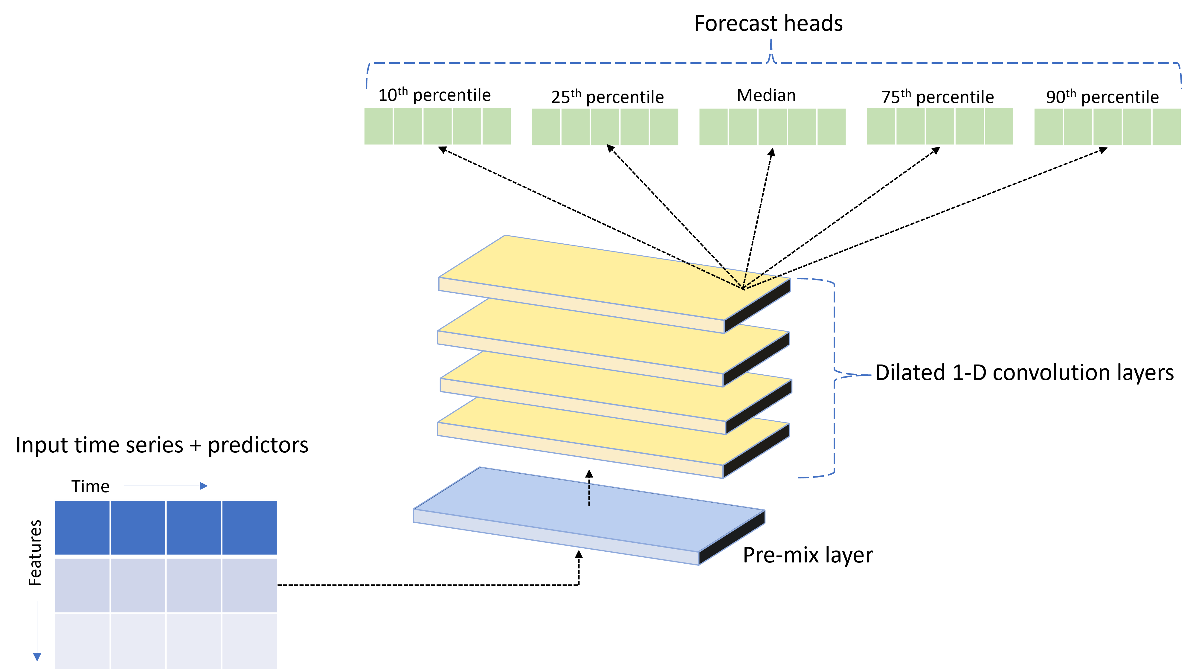
TCNForecaster has the following main components:

• A pre-mix layer that mixes the input time series and feature data into an array of signal channels that the convolutional stack will process.
• A stack of dilated convolution layers that processes the channel array sequentially; each layer in the stack processes the output of the previous layer to produce a new channel array. Each channel in this output contains a mixture of convolution-filtered signals from the input channels.
• A collection of forecast head units that coalesce the output signals from the convolution layers and generate forecasts of the target quantity from this latent representation. Each head unit produces forecasts up to the horizon for a quantile of the prediction distribution.

Dilated causal convolution

The central operation of a TCN is a dilated, causal convolution along the time dimension of an input signal. Intuitively, convolution mixes together values from nearby time points in the input. The proportions in the mixture are the kernel, or the weights, of the convolution while the separation between points in the mixture is the dilation. The output signal is generated from the input by sliding the kernel in time along the input and accumulating the mixture at each position. A causal convolution is one in which the kernel only mixes input values in the past relative to each output point, preventing the output from "looking" into the future.

Stacking dilated convolutions gives the TCN the ability to model correlations over long durations in input signals with relatively few kernel weights. For example, the following image shows three stacked layers with a two-weight kernel in each layer and exponentially increasing dilation factors:

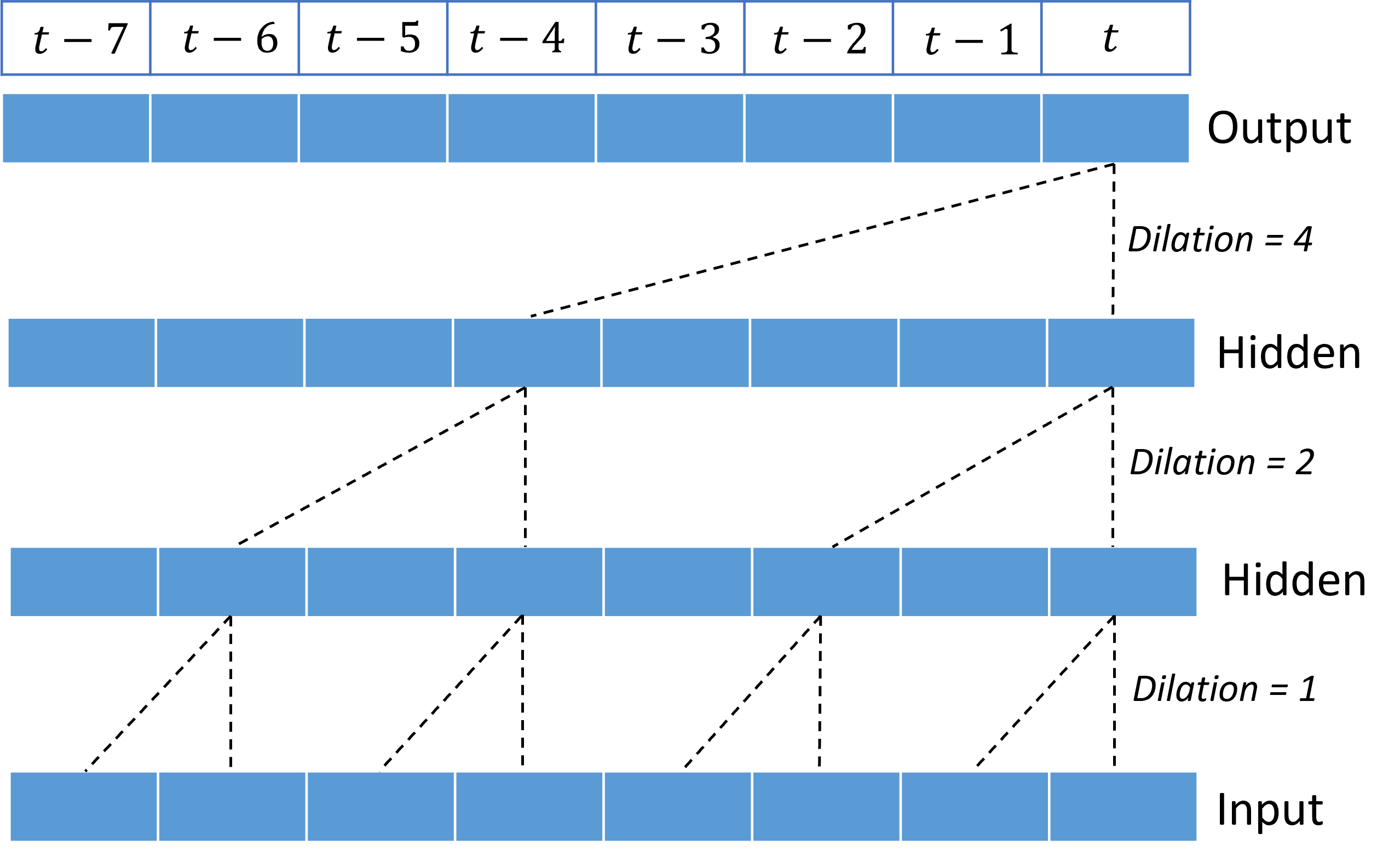
The dashed lines show paths through the network that end on the output at a time $t$. These paths cover the last eight points in the input, illustrating that each output point is a function of the eight most relatively recent points in the input. The length of history, or "look back," that a convolutional network uses to make predictions is called the receptive field and it is determined completely by the TCN architecture.

TCNForecaster architecture

The core of the TCNForecaster architecture is the stack of convolutional layers between the pre-mix and the forecast heads. The stack is logically divided into repeating units called blocks that are, in turn, composed of residual cells. A residual cell applies causal convolutions at a set dilation along with normalization and nonlinear activation. Importantly, each residual cell adds its output to its input using a so-called residual connection. These connections have been shown to benefit DNN training, perhaps because they facilitate more efficient information flow through the network. The following image shows the architecture of the convolutional layers for an example network with two blocks and three residual cells in each block:

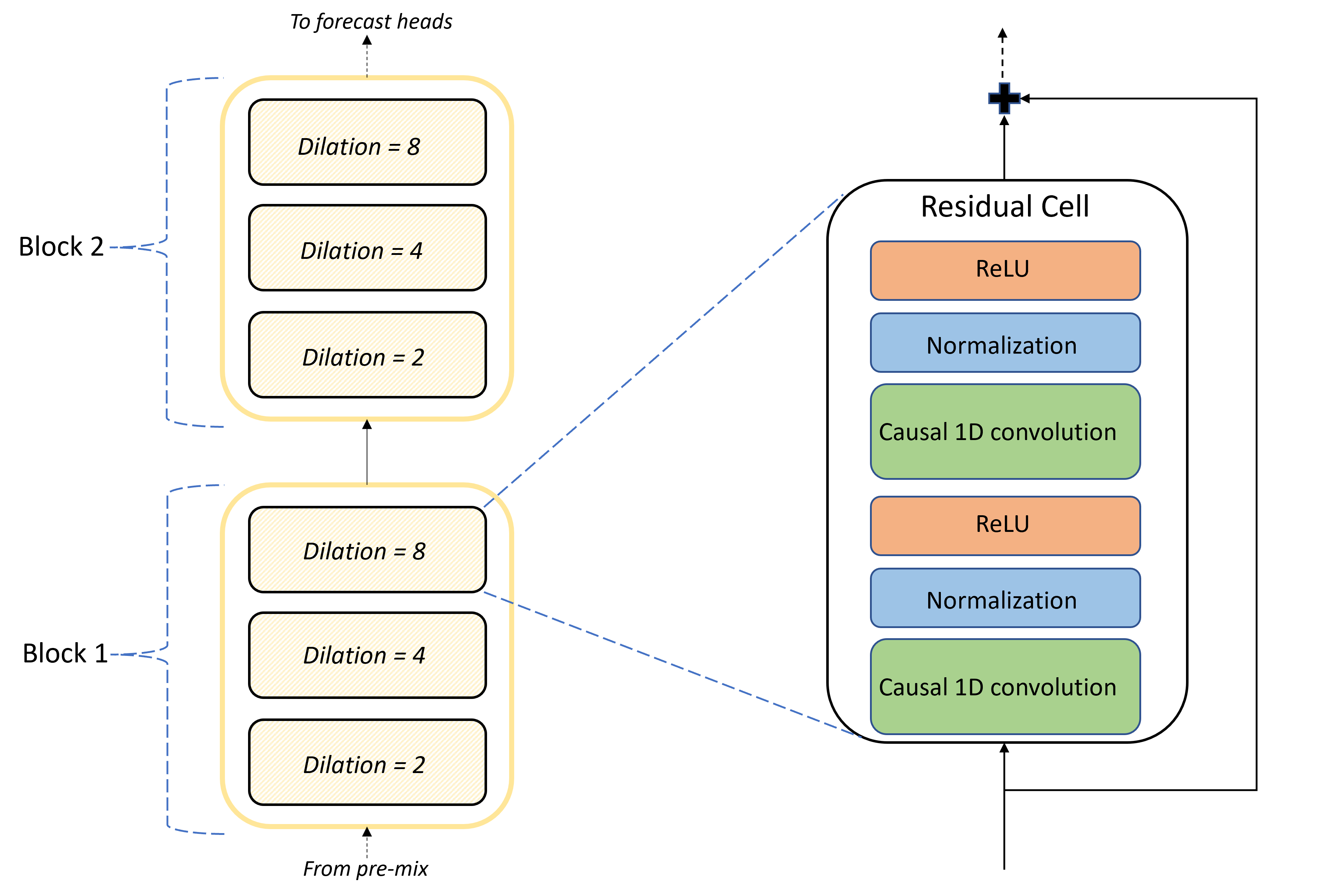
The number of blocks and cells, along with the number of signal channels in each layer, control the size of the network. The architectural parameters of TCNForecaster are summarized in the following table:

Parameter	Description
$n_{b}$	Number of blocks in the network; also called the depth
$n_{c}$	Number of cells in each block
$n_{\text{ch}}$	Number of channels in the hidden layers

The receptive field depends on the depth parameters and is given by the formula,

$t_{\text{rf}} = 4n_{b}\left(2^{n_{c}} - 1\right) + 1.$

We can give a more precise definition of the TCNForecaster architecture in terms of formulas. Let $X$ be an input array where each row contains feature values from the input data. We can divide $X$ into numeric and categorical feature arrays, $X_{\text{num}}$ and $X_{\text{cat}}$. Then, the TCNForecaster is given by the formulas,

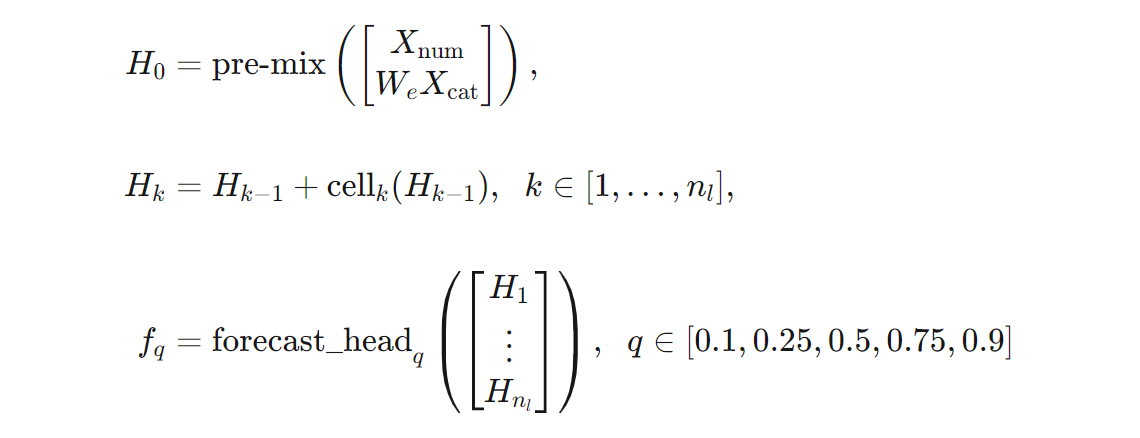
where $W_{e}$ is an embedding matrix for the categorical features, $n_{l} = n_{b}n_{c}$ is the total number of residual cells, the $H_{k}$ denote hidden layer outputs, and the $f_{q}$ are forecast outputs for given quantiles of the prediction distribution. To aid understanding, the dimensions of these variables are in the following table:

Variable	Description	Dimensions
$X$	Input array	$n_{\text{input}} \times t_{\text{rf}}$
$H_{i}$	Hidden layer output for $i=0,1,\ldots,n_{l}$	$n_{\text{ch}} \times t_{\text{rf}}$
$f_{q}$	Forecast output for quantile $q$	$h$

In the table, $n_{\text{input}} = n_{\text{features}} + 1$, the number of predictor/feature variables plus the target quantity. The forecast heads generate all forecasts up to the maximum horizon, $h$, in a single pass, so TCNForecaster is a direct forecaster.

TCNForecaster in AutoML

TCNForecaster is an optional model in AutoML. To learn how to use it, see enable deep learning.

In this section, we'll describe how AutoML builds TCNForecaster models with your data, including explanations of data preprocessing, training, and model search.

Data preprocessing steps

AutoML executes several preprocessing steps on your data to prepare for model training. The following table describes these steps in the order they're performed:

Step	Description
Fill missing data	Impute missing values and observation gaps and optionally pad or drop short time series
Create calendar features	Augment the input data with features derived from the calendar like day of the week and, optionally, holidays for a specific country/region.
Encode categorical data	Label encode strings and other categorical types; this includes all time series ID columns.
Target transform	Optionally apply the natural logarithm function to the target depending on the results of certain statistical tests.
Normalization	Z-score normalize all numeric data; normalization is performed per feature and per time series group, as defined by the time series ID columns.

These steps are included in AutoML's transform pipelines, so they are automatically applied when needed at inference time. In some cases, the inverse operation to a step is included in the inference pipeline. For example, if AutoML applied a $\log$ transform to the target during training, the raw forecasts are exponentiated in the inference pipeline.

Training

The TCNForecaster follows DNN training best practices common to other applications in images and language. AutoML divides preprocessed training data into examples that are shuffled and combined into batches. The network processes the batches sequentially, using back propagation and stochastic gradient descent to optimize the network weights with respect to a loss function. Training can require many passes through the full training data; each pass is called an epoch.

The following table lists and describes input settings and parameters for TCNForecaster training:

Training input	Description	Value
Validation data	A portion of data that is held out from training to guide the network optimization and mitigate over fitting.	Provided by the user or automatically created from training data if not provided.
Primary metric	Metric computed from median-value forecasts on the validation data at the end of each training epoch; used for early stopping and model selection.	Chosen by the user; normalized root mean squared error or normalized mean absolute error.
Training epochs	Maximum number of epochs to run for network weight optimization.	100; automated early stopping logic may terminate training at a smaller number of epochs.
Early stopping patience	Number of epochs to wait for primary metric improvement before training is stopped.	20
Loss function	The objective function for network weight optimization.	Quantile loss averaged over 10th, 25th, 50th, 75th, and 90th percentile forecasts.
Batch size	Number of examples in a batch. Each example has dimensions $n_{\text{input}} \times t_{\text{rf}}$ for input and $h$ for output.	Determined automatically from the total number of examples in the training data; maximum value of 1024.
Embedding dimensions	Dimensions of the embedding spaces for categorical features.	Automatically set to the fourth root of the number of distinct values in each feature, rounded up to the closest integer. Thresholds are applied at a minimum value of 3 and maximum value of 100.
Network architecture*	Parameters that control the size and shape of the network: depth, number of cells, and number of channels.	Determined by model search.
Network weights	Parameters controlling signal mixtures, categorical embeddings, convolution kernel weights, and mappings to forecast values.	Randomly initialized, then optimized with respect to the loss function.
Learning rate*	Controls how much the network weights can be adjusted in each iteration of gradient descent; dynamically reduced near convergence.	Determined by model search.
Dropout ratio*	Controls the degree of dropout regularization applied to the network weights.	Determined by model search.

Inputs marked with an asterisk (*) are determined by a hyper-parameter search that is described in the next section.

Model search

AutoML uses model search methods to find values for the following hyper-parameters:

• Network depth, or the number of convolutional blocks,
• Number of cells per block,
• Number of channels in each hidden layer,
• Dropout ratio for network regularization,
• Learning rate.

Optimal values for these parameters can vary significantly depending on the problem scenario and training data, so AutoML trains several different models within the space of hyper-parameter values and picks the best one according to the primary metric score on the validation data.

The model search has two phases:

1. AutoML performs a search over 12 "landmark" models. The landmark models are static and chosen to reasonably span the hyper-parameter space.
2. AutoML continues searching through the hyper-parameter space using a random search.

The search terminates when stopping criteria are met. The stopping criteria depend on the forecast training job configuration, but some examples include time limits, limits on number of search trials to perform, and early stopping logic when the validation metric is not improving.

Next steps

• Learn how to set up AutoML to train a time-series forecasting model.
• Learn about forecasting methodology in AutoML.
• Browse frequently asked questions about forecasting in AutoML.