Feature transformation and best practices

This article describes feature set specifications, the different kinds of transformations that can be used with it, and related best practices.

A feature set is a collection of features generated by source data transformations. A feature set specification is a self-contained definition for feature set development and local testing. After its development and local testing, you can register that feature set as a feature set asset with the feature store. You then have versioning and materialization available as managed capabilities.

Define a feature set

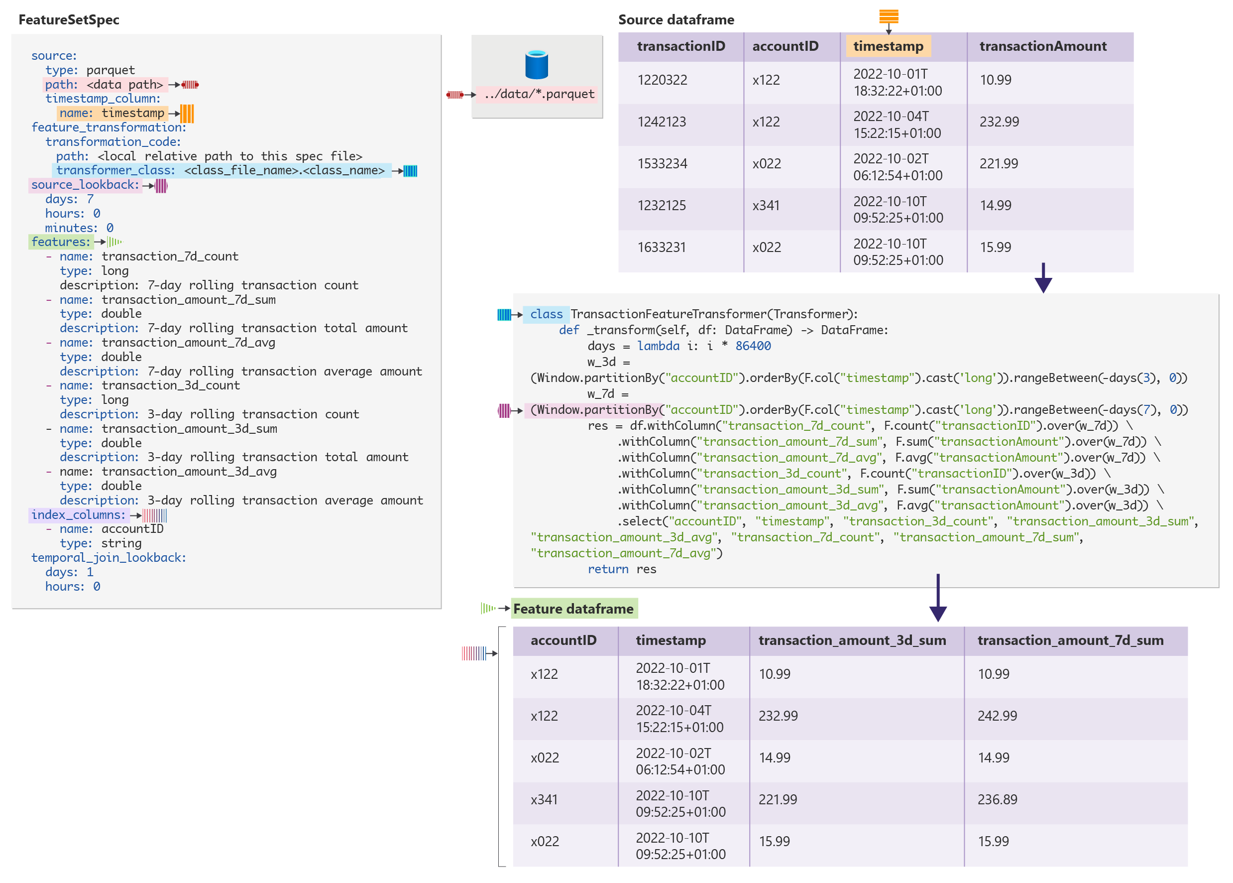
FeatureSetSpec defines a feature set. This sample shows a feature set specification file:

$schema: http://azureml/sdk-2-0/FeatureSetSpec.json

source:
  type: parquet
  path: abfs://file_system@account_name.dfs.core.windows.net/datasources/transactions-source/*.parquet
  timestamp_column: # name of the column representing the timestamp.
    name: timestamp
  source_delay:
    days: 0
    hours: 3
    minutes: 0
feature_transformation:
  transformation_code:
    path: ./transformation_code
    transformer_class: transaction_transform.TransactionFeatureTransformer
features:
  - name: transaction_7d_count
    type: long
  - name: transaction_amount_7d_sum
    type: double
  - name: transaction_amount_7d_avg
    type: double
  - name: transaction_3d_count
    type: long
  - name: transaction_amount_3d_sum
    type: double
  - name: transaction_amount_3d_avg
    type: double
index_columns:
  - name: accountID
    type: string
source_lookback:
  days: 7
  hours: 0
  minutes: 0
temporal_join_lookback:
  days: 1
  hours: 0
  minutes: 0

Note

The featurestore core SDK autogenerates the feature set specification YAML. This tutorial has an example.

In the FeatureSetSpec definition, these properties have relevance to feature transformation:

• source: defines the source data and relevant metadata - for example, the timestamp column in the data. Currently, only time-series source data and features are supported. The source.timestamp_column property is mandatory
• feature_transformation.transformation_code: defines the code folder location of the feature transformer
• features: defines the feature schema generated by the feature transformer
• index_columns: defines the index column(s) schema that the feature transformer generates
• source_lookback: this property is used when the feature handles aggregation on time-series (for example, window aggregation) data. The value of this property indicates the required time range of source data in the past, for a feature value at time T. The Best Practice section has details.

How are features calculated?

After you define a FeatureSetSpec, invoke featureSetSpec.to_spark_dataframe(feature_window_start_ts, feature_window_end_ts) to calculate features on a given feature window.

The calculation happens in these steps:

• Read data from the source data. The source defines the source data. Filter the data by the time range [feature_window_start_ts - source_lookback, feature_window_end_ts). The time range includes the start of the window, and excludes the end of the window
• Apply the feature transformer, defined by feature_transformation.transformation_code, on the data, and get the calculated features
• Filter the feature values to return only those feature records within the feature window [feature_window_start_ts, feature_window_end_ts)

In this code sample, the feature store API computes the features:

# define the source data time window according to feature window
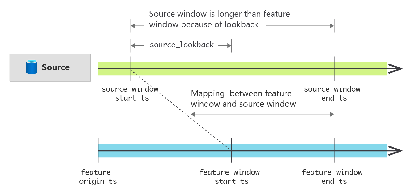
source_window_start_ts = feature_window_start_ts - source_lookback
source_window_end_ts = feature_window_end_ts

# read source table into a dataframe
df1 = spark.read.parquet(source.path).filter(df1["timestamp"] >= source_window_start_ts && df1["timestamp"] < source_window_end_ts)

# apply the feature transformer
df2 = FeatureTransformer._transform(df1)

## filter the feature(set) to include only feature records within the feature window
feature_set_df = df2.filter(df2["timestamp"] >= feature_window_start_ts && df2["timestamp"] < feature_window_end_ts)

Output schema of the feature transformer function

The transform function outputs a dataframe, which includes these values in its schema:

• Index columns that match the FeatureSetSpec definition, both in name and type
• The timestamp column (name) that matches the timestamp definition in the source. The source is found in FeatureSetSpec
• Define all other column name/type values as features in FeatureSetSpec

Implement feature transformer for common types of transformations

Row-level transformation

In a row-level transformation, a feature value calculation on a specific row only uses column values of that row. Start with this source data:

user_id	timestamp	total_spend
1	2022-12-19 06:00:00	12.00
2	2022-12-10 03:00:00	56.00
1	2022-12-25 13:00:00	112.00

Define a new feature set named user_total_spend_profile:

from pyspark.sql import Dataframe
from pyspark.ml import Transformer

class UserTotalSpendProfileTransformer(Transformer):

    def _transform(df: Dataframe) -> Dataframe:
        df.withColumn("is_high_spend_user", col("total_spend") > 100.0) \
           .withColumn("is_low_spend_user", col("total_spend") < 20.0)

This feature set has three features, with data types as shown:

• total_spend: double
• is_high_spend_user: bool
• is_low_spend_user: bool

This shows the calculated feature values:

user_id	timestamp	total_spend	is_high_spend_user	is_low_spend_user
1	2022-12-19 06:00:00	12.00	false	true
2	2022-12-10 03:00:00	56.00	false	false
1	2022-12-25 13:00:00	112.00	true	false

Sliding window aggregation

Sliding window aggregation can help handle feature values that present statistics (for example, sum, average, etc.) that accumulate over time. The SparkSQL Window function defines a sliding window around each row in the data, is useful in these cases.

For each row, the Window object can look into both future and past. In the context of machine learning features, you should define the Window object to look only the past, for each row. Visit the Best Practice section for more details.

Start with this source data:

user_id	timestamp	spend
1	2022-12-10 06:00:00	12.00
2	2022-12-10 03:00:00	56.00
1	2022-12-11 01:00:00	10.00
2	2022-12-11 20:00:00	10.00
2	2022-12-12 02:00:00	100.00

Define a new feature set named user_rolling_spend. This feature set includes rolling 1-day and 3-day total spending, by user:

from pyspark.sql import Dataframe
from pyspark.sql import functions as F
from pyspark.sql.window import Window
from pyspark.ml import Transformer

class UserRollingSpend(Transformer):

    def _transform(df: Dataframe) -> Dataframe:
        days = lambda i: i * 86400
        w_1d = (Window.partitionBy("user_id").orderBy(F.col("timestamp").cast('long'))\
                .rangeBetween(-days(1), 0))
        w_3d = (Window.partitionBy("user_id").orderBy(F.col("timestamp").cast('long')).\
                rangeBetween(-days(3), 0))
        res = df.withColumn("spend_1d_sum", F.sum("spend").over(w_1d)) \
            .withColumn("spend_3d_sum", F.sum("spend").over(w_3d)) \
            .select("user_id", "timestamp", "spend_1d_sum", "spend_3d_sum")
        return res
    

The user_rolling_spend feature set has two features:

• spend_1d_sum: double
• spend_3d_sum: double

This shows its calculated feature values:

user_id	timestamp	spend_1d_sum	spend_3d_sum
1	2022-12-10 06:00:00	12.00	12.00
2	2022-12-10 03:00:00	56.00	56.00
1	2022-12-11 01:00:00	22.00	22.00
2	2022-12-11 20:00:00	10.00	66.00
2	2022-12-12 02:00:00	110.00	166.00

The feature value calculations use columns on the current row, combined with preceding row columns within the range.

Tumbling window aggregation

A tumbling window can aggregate data on time-series data. Group the data into fixed-size, nonoverlapping and continuous time windows, and then aggregate it. For example, users can define features based on daily or hourly aggregation. Use the pyspark.sql.functions.window function to define a tumbling window, for consistent results. The output feature timestamp should align with the end of each tumbling window.

Start with this source data:

user_id	timestamp	spend
1	2022-12-10 06:00:00	12.00
1	2022-12-10 16:00:00	10.00
2	2022-12-10 03:00:00	56.00
1	2022-12-11 01:00:00	10.00
2	2022-12-12 04:00:00	23.00
2	2022-12-12 12:00:00	10.00

Define a new feature set named user_daily_spend:

from pyspark.sql import functions as F
from pyspark.ml import Transformer
from pyspark.sql.dataframe import DataFrame

class TransactionFeatureTransformer(Transformer):
    def _transform(self, df: DataFrame) -> DataFrame:
        df1 = df.groupBy("user_id", F.window("timestamp", windowDuration="1 day",slideDuration="1 day"))\
                .agg(F.sum("spend").alias("daily_spend"))
        df2 = df1.select("user_id", df1.window.end.cast("timestamp").alias("end"),"daily_spend")
        df3 = df2.withColumn('timestamp', F.expr("end - INTERVAL 1 milliseconds")) \
              .select("user_id", "timestamp","daily_spend")
        return df3

The user_daily_spend feature set has this feature:

• daily_spend: double

This shows its calculated feature values:

user_id	timestamp	daily_spend
1	2022-12-10 23:59:59	22.00
2	2022-12-10 23:59:59	56.00
1	2022-12-11 23:59:59	10.00
2	2022-12-12 23:59:59	33.00

Stagger window aggregation

Stagger window aggregation is a minor variant of the tumbling window aggregation. Stagger window aggregation groups the data into fixed-size windows. However, the windows can overlap each other. For this, use pyspark.sql.functions.window, with a slideDuration smaller than windowDuration.

Start with this example data:

user_id	timestamp	spend
1	2022-12-10 03:00:00	12.00
1	2022-12-10 09:00:00	10.00
1	2022-12-11 05:00:00	8.00
2	2022-12-12 14:00:00	56.00

Define a new feature set named user_sliding_24hr_spend:

from pyspark.sql import functions as F
from pyspark.ml import Transformer
from pyspark.sql.dataframe import DataFrame

class TrsactionFeatureTransformer(Transformer):
    def _transform(self, df: DataFrame) -> DataFrame:
        df1 = df.groupBy("user_id", F.window("timestamp", windowDuration="1 day",slideDuration="6 hours"))\
                .agg(F.sum("spend").alias("sliding_24hr_spend"))
        df2 = df1.select("user_id", df1.window.end.cast("timestamp").alias("end"),"sliding_24hr_spend")
        df3 = df2.withColumn('timestamp', F.expr("end - INTERVAL 1 milliseconds")) \
              .select("user_id", "timestamp","sliding_24hr_spend")
        return df3

The user_sliding_24hr_spend feature set has one feature:

• sliding_24hr_spend: double

This shows its calculated feature values:

user_id	timestamp	sliding_24hr_spend
1	2022-12-10 05:59:59	12.00
1	2022-12-10 11:59:59	22.00
1	2022-12-10 17:59:59	22.00
1	2022-12-10 23:59:59	22.00
1	2022-12-11 05:59:59	18.00
1	2022-12-11 11:59:59	8.00
1	2022-12-11 17:59:59	8.00
1	2022-12-11 23:59:59	8.00
1	2022-12-12 05:59:59	18.00
2	2022-12-12 17:59:59	56.00
2	2022-12-12 23:59:59	56.00
2	2022-12-13 05:59:59	56.00
2	2022-12-13 11:59:59	56.00

Define feature transformations - best practices

Prevent data leakage in feature transformation

If the timestamp value for each calculated feature value is ts_0, calculate the feature values based on source data with timestamp values on or before ts_0 only. This avoids feature calculation based on data from after the feature event time, otherwise known as data leakage.

Data leakage usually happens with sliding/tumbling/stagger window aggregation. These best practices can help avoid leakage:

• Sliding window aggregation: define the window to look only back in time, from each row
• Tumbling/stagger window aggregation: define the feature timestamp based on the end of each window

This data sample shows good and bad example data:

Aggregation	Good example	Bad example with data leakage
Sliding window	Window.partitionBy("user_id") .orderBy(F.col("timestamp").cast('long')) .rangeBetween(-days(4), 0)	Window.partitionBy("user_id") .orderBy(F.col("timestamp").cast('long')) .rangeBetween(-days(2), days(2))
Tumbling/stagger window	df1 = df.groupBy("user_id", F.window("timestamp", windowDuration="1 day",slideDuration="1 day")) .agg(F.sum("spend").alias("daily_spend")) df2 = df1.select("user_id", df1.window.end.cast("timestamp").alias("timestamp"),"daily_spend")	df1 = df.groupBy("user_id", F.window("timestamp", windowDuration="1 day",slideDuration="1 day")) .agg(F.sum("spend").alias("daily_spend")) df2 = df1.select("user_id", df1.window.start.cast("timestamp").alias("timestamp"),"daily_spend")

Data leakage in the feature transformation definition can lead to these problems:

• Errors in the calculated/materialized feature values
• Inconsistencies in get_offline_feature, when using the materialized feature value instead of values calculated on the fly

Set proper source_lookback

For time-series (sliding/tumbling/stagger window aggregation) data aggregations, properly set the source_lookback property. This diagram shows the relationship between the source data window and the feature window in the feature (set) calculation:

Define source_lookback as a time delta value, which presents the range of source data needed for a feature value of a given timestamp. This example shows the recommended source_lookback values for the common transformation types:

Transformation type	source_lookback
Row-level transformation	0 (default)
Sliding window	size of the largest window range in the transformer. e.g. source_lookback = 3 days when the feature set defines 3 day rolling features source_lookback = 7 days when the feature set defines both 3 day and 7 day rolling features
Tumbling/stagger window	value of windowDuration in window definition. e.g. source_lookback = 1day when using window("timestamp", windowDuration="1 day",slideDuration="6 hours)

Incorrect source_lookback settings can lead to incorrect calculated/materialized feature values.

Next steps

• Tutorial 1: Develop and register a feature set with managed feature store
• GitHub Sample Repository