Tutorial: Train and deploy an image classification model with an example Jupyter Notebook

Article
04/02/2024

In this tutorial, you train a machine learning model on remote compute resources. You use the training and deployment workflow for Azure Machine Learning in a Python Jupyter Notebook. You can then use the notebook as a template to train your own machine learning model with your own data.

This tutorial trains a simple logistic regression by using the MNIST dataset and scikit-learn with Azure Machine Learning. MNIST is a popular dataset consisting of 70,000 grayscale images. Each image is a handwritten digit of 28 x 28 pixels, representing a number from zero to nine. The goal is to create a multi-class classifier to identify the digit a given image represents.

Learn how to take the following actions:

Download a dataset and look at the data.
Train an image classification model and log metrics using MLflow.
Deploy the model to do real-time inference.

Prerequisites

Complete the Quickstart: Get started with Azure Machine Learning to:
- Create a workspace.
- Create a cloud-based compute instance to use for your development environment.

Run a notebook from your workspace

Azure Machine Learning includes a cloud notebook server in your workspace for an install-free and preconfigured experience. Use your own environment if you prefer to have control over your environment, packages, and dependencies.

Clone a notebook folder

You complete the following experiment setup and run steps in Azure Machine Learning studio. This consolidated interface includes machine learning tools to perform data science scenarios for data science practitioners of all skill levels.

Sign in to Azure Machine Learning studio.
Select your subscription and the workspace you created.
On the left, select Notebooks.
At the top, select the Samples tab.
Open the SDK v1 folder.
Select the ... button at the right of the tutorials folder, and then select Clone.
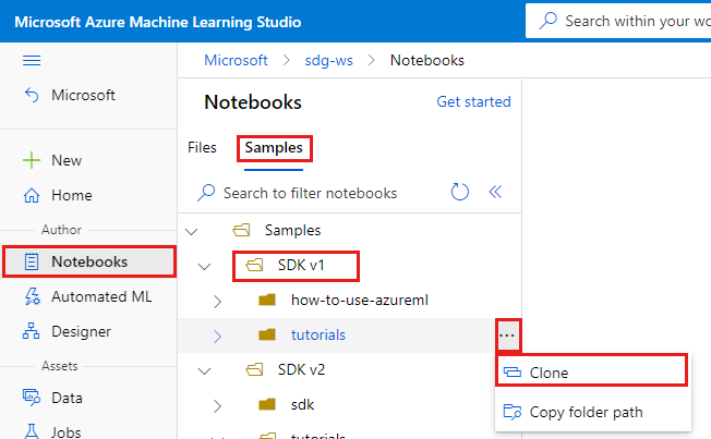
A list of folders shows each user who accesses the workspace. Select your folder to clone the tutorials folder there.

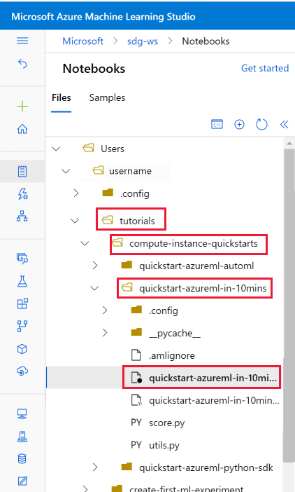
Open the cloned notebook

Open the tutorials folder that was cloned into your User files section.
Select the quickstart-azureml-in-10mins.ipynb file from your tutorials/compute-instance-quickstarts/quickstart-azureml-in-10mins folder.

Install packages

Once the compute instance is running and the kernel appears, add a new code cell to install packages needed for this tutorial.

At the top of the notebook, add a code cell.
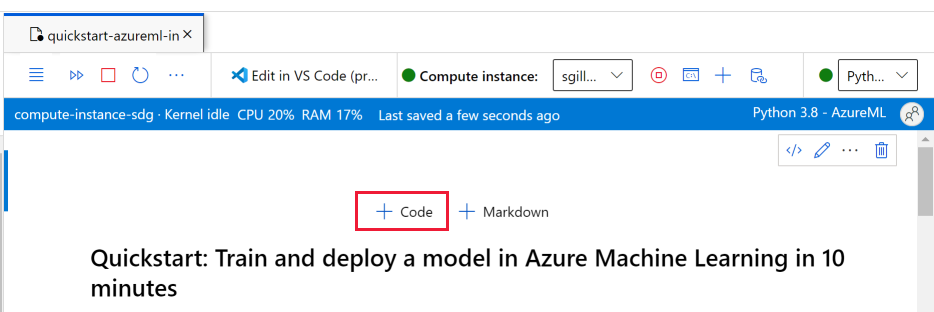
Add the following into the cell and then run the cell, either by using the Run tool or by using Shift+Enter.
```
%pip install scikit-learn==0.22.1
%pip install scipy==1.5.2
```

You may see a few install warnings. These can safely be ignored.

Run the notebook

This tutorial and accompanying utils.py file is also available on GitHub if you wish to use it on your own local environment. If you aren't using the compute instance, add %pip install azureml-sdk[notebooks] azureml-opendatasets matplotlib to the install above.

Important

The rest of this article contains the same content as you see in the notebook.

Switch to the Jupyter Notebook now if you want to run the code while you read along. To run a single code cell in a notebook, click the code cell and hit Shift+Enter. Or, run the entire notebook by choosing Run all from the top toolbar.

Import data

Before you train a model, you need to understand the data you're using to train it. In this section, learn how to:

Download the MNIST dataset
Display some sample images

You use Azure Open Datasets to get the raw MNIST data files. Azure Open Datasets are curated public datasets that you can use to add scenario-specific features to machine learning solutions for better models. Each dataset has a corresponding class, MNIST in this case, to retrieve the data in different ways.

import os
from azureml.opendatasets import MNIST

data_folder = os.path.join(os.getcwd(), "/tmp/qs_data")
os.makedirs(data_folder, exist_ok=True)

mnist_file_dataset = MNIST.get_file_dataset()
mnist_file_dataset.download(data_folder, overwrite=True)

Take a look at the data

Load the compressed files into numpy arrays. Then use matplotlib to plot 30 random images from the dataset with their labels above them.

Note this step requires a load_data function, included in an utils.py file. This file is placed in the same folder as this notebook. The load_data function simply parses the compressed files into numpy arrays.

from utils import load_data
import matplotlib.pyplot as plt
import numpy as np
import glob


# note we also shrink the intensity values (X) from 0-255 to 0-1. This helps the model converge faster.
X_train = (
    load_data(
        glob.glob(
            os.path.join(data_folder, "**/train-images-idx3-ubyte.gz"), recursive=True
        )[0],
        False,
    )
    / 255.0
)
X_test = (
    load_data(
        glob.glob(
            os.path.join(data_folder, "**/t10k-images-idx3-ubyte.gz"), recursive=True
        )[0],
        False,
    )
    / 255.0
)
y_train = load_data(
    glob.glob(
        os.path.join(data_folder, "**/train-labels-idx1-ubyte.gz"), recursive=True
    )[0],
    True,
).reshape(-1)
y_test = load_data(
    glob.glob(
        os.path.join(data_folder, "**/t10k-labels-idx1-ubyte.gz"), recursive=True
    )[0],
    True,
).reshape(-1)


# now let's show some randomly chosen images from the traininng set.
count = 0
sample_size = 30
plt.figure(figsize=(16, 6))
for i in np.random.permutation(X_train.shape[0])[:sample_size]:
    count = count + 1
    plt.subplot(1, sample_size, count)
    plt.axhline("")
    plt.axvline("")
    plt.text(x=10, y=-10, s=y_train[i], fontsize=18)
    plt.imshow(X_train[i].reshape(28, 28), cmap=plt.cm.Greys)
plt.show()

The code displays a random set of images with their labels, similar to this:

Sample images with their labels.

Train model and log metrics with MLflow

Train the model using the following code. This code uses MLflow autologging to track metrics and log model artifacts.

You'll be using the LogisticRegression classifier from the SciKit Learn framework to classify the data.

Note

The model training takes approximately 2 minutes to complete.

# create the model
import mlflow
import numpy as np
from sklearn.linear_model import LogisticRegression
from azureml.core import Workspace

# connect to your workspace
ws = Workspace.from_config()

# create experiment and start logging to a new run in the experiment
experiment_name = "azure-ml-in10-mins-tutorial"

# set up MLflow to track the metrics
mlflow.set_tracking_uri(ws.get_mlflow_tracking_uri())
mlflow.set_experiment(experiment_name)
mlflow.autolog()

# set up the Logistic regression model
reg = 0.5
clf = LogisticRegression(
    C=1.0 / reg, solver="liblinear", multi_class="auto", random_state=42
)

# train the model
with mlflow.start_run() as run:
    clf.fit(X_train, y_train)

View experiment

In the left-hand menu in Azure Machine Learning studio, select Jobs and then select your job (azure-ml-in10-mins-tutorial). A job is a grouping of many runs from a specified script or piece of code. Multiple jobs can be grouped together as an experiment.

Information for the run is stored under that job. If the name doesn't exist when you submit a job, if you select your run you'll see various tabs containing metrics, logs, explanations, etc.

Version control your models with the model registry

You can use model registration to store and version your models in your workspace. Registered models are identified by name and version. Each time you register a model with the same name as an existing one, the registry increments the version. The code below registers and versions the model you trained above. Once you execute the following code cell, you'll see the model in the registry by selecting Models in the left-hand menu in Azure Machine Learning studio.

# register the model
model_uri = "runs:/{}/model".format(run.info.run_id)
model = mlflow.register_model(model_uri, "sklearn_mnist_model")

Deploy the model for real-time inference

In this section, learn how to deploy a model so that an application can consume (inference) the model over REST.

Create deployment configuration

The code cell gets a curated environment, which specifies all the dependencies required to host the model (for example, the packages like scikit-learn). Also, you create a deployment configuration, which specifies the amount of compute required to host the model. In this case, the compute has 1CPU and 1-GB memory.

# create environment for the deploy
from azureml.core.environment import Environment
from azureml.core.conda_dependencies import CondaDependencies
from azureml.core.webservice import AciWebservice

# get a curated environment
env = Environment.get(
    workspace=ws, 
    name="AzureML-sklearn-1.0"
)
env.inferencing_stack_version='latest'

# create deployment config i.e. compute resources
aciconfig = AciWebservice.deploy_configuration(
    cpu_cores=1,
    memory_gb=1,
    tags={"data": "MNIST", "method": "sklearn"},
    description="Predict MNIST with sklearn",
)

Deploy model

This next code cell deploys the model to Azure Container Instance.

Note

The deployment takes approximately 3 minutes to complete. But it might be longer to until it is available for use, perhaps as long as 15 minutes.**

%%time
import uuid
from azureml.core.model import InferenceConfig
from azureml.core.environment import Environment
from azureml.core.model import Model

# get the registered model
model = Model(ws, "sklearn_mnist_model")

# create an inference config i.e. the scoring script and environment
inference_config = InferenceConfig(entry_script="score.py", environment=env)

# deploy the service
service_name = "sklearn-mnist-svc-" + str(uuid.uuid4())[:4]
service = Model.deploy(
    workspace=ws,
    name=service_name,
    models=[model],
    inference_config=inference_config,
    deployment_config=aciconfig,
)

service.wait_for_deployment(show_output=True)

The scoring script file referenced in the preceding code can be found in the same folder as this notebook, and has two functions:

An init function that executes once when the service starts - in this function you normally get the model from the registry and set global variables
A run(data) function that executes each time a call is made to the service. In this function, you normally format the input data, run a prediction, and output the predicted result.

View endpoint

Once the model is successfully deployed, you can view the endpoint by navigating to Endpoints in the left-hand menu in Azure Machine Learning studio. You'll see the state of the endpoint (healthy/unhealthy), logs, and consume (how applications can consume the model).

Test the model service

You can test the model by sending a raw HTTP request to test the web service.

# send raw HTTP request to test the web service.
import requests

# send a random row from the test set to score
random_index = np.random.randint(0, len(X_test) - 1)
input_data = '{"data": [' + str(list(X_test[random_index])) + "]}"

headers = {"Content-Type": "application/json"}

resp = requests.post(service.scoring_uri, input_data, headers=headers)

print("POST to url", service.scoring_uri)
print("label:", y_test[random_index])
print("prediction:", resp.text)

Clean up resources

If you're not going to continue to use this model, delete the Model service using:

# if you want to keep workspace and only delete endpoint (it will incur cost while running)
service.delete()

If you want to control cost further, stop the compute instance by selecting the "Stop compute" button next to the Compute dropdown. Then start the compute instance again the next time you need it.

Delete everything

Use these steps to delete your Azure Machine Learning workspace and all compute resources.

Important

The resources that you created can be used as prerequisites to other Azure Machine Learning tutorials and how-to articles.

If you don't plan to use any of the resources that you created, delete them so you don't incur any charges:

In the Azure portal, select Resource groups on the far left.
From the list, select the resource group that you created.
Select Delete resource group.
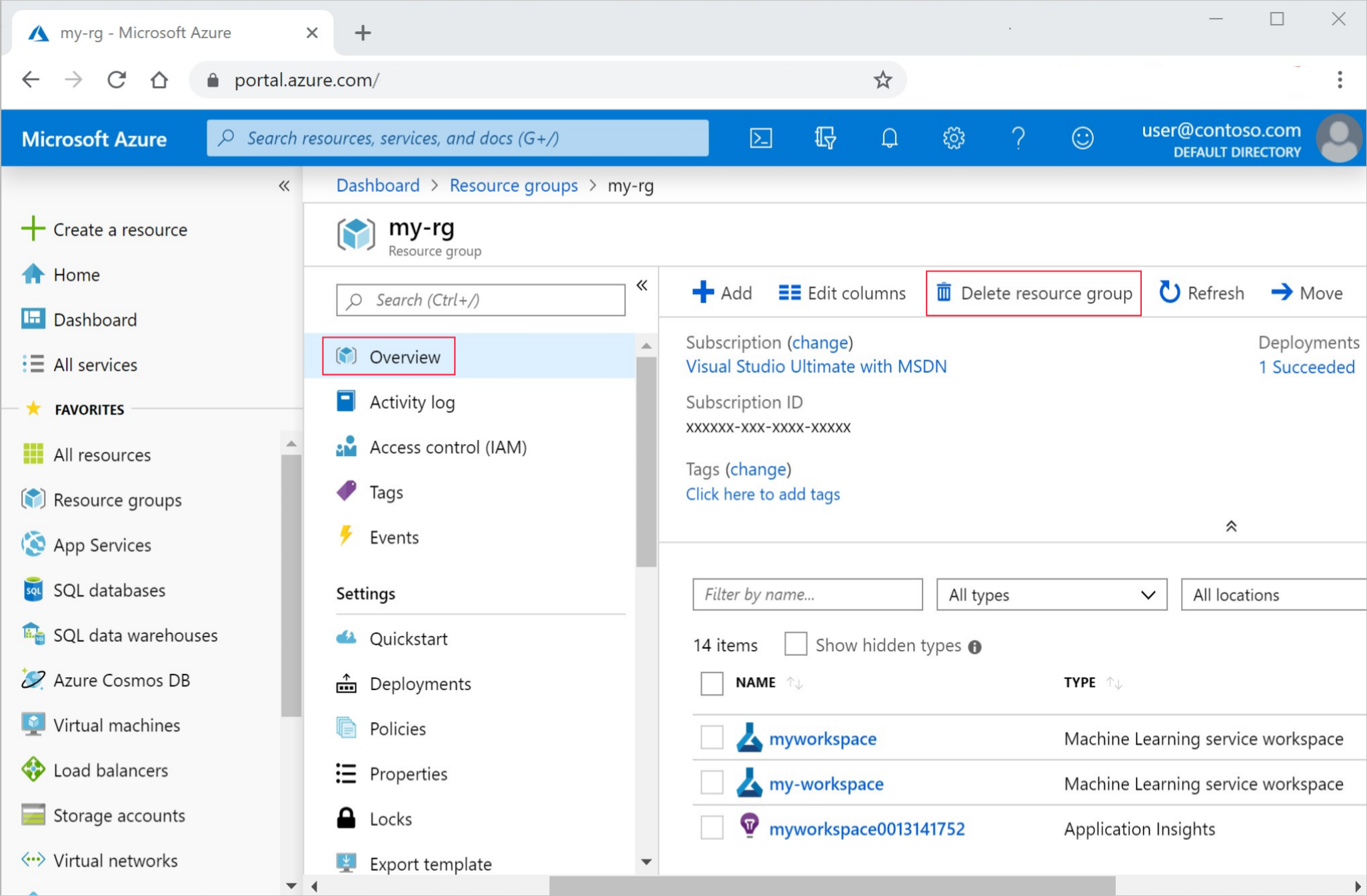
Enter the resource group name. Then select Delete.

Learn about all of the deployment options for Azure Machine Learning.
Learn how to authenticate to the deployed model.
Make predictions on large quantities of data asynchronously.
Monitor your Azure Machine Learning models with Application Insights.

Tutorial: Train and deploy an image classification model with an example Jupyter Notebook

Prerequisites

Run a notebook from your workspace

Clone a notebook folder

Open the cloned notebook

Install packages

Run the notebook

Import data

Take a look at the data

Train model and log metrics with MLflow

View experiment

Version control your models with the model registry

Deploy the model for real-time inference

Create deployment configuration

Deploy model

View endpoint

Test the model service

Clean up resources

Delete everything

Feedback

Additional resources

Tutorial: Train and deploy an image classification model with an example Jupyter Notebook

Prerequisites

Run a notebook from your workspace

Clone a notebook folder

Open the cloned notebook

Install packages

Run the notebook

Import data

Take a look at the data

Train model and log metrics with MLflow

View experiment

Version control your models with the model registry

Deploy the model for real-time inference

Create deployment configuration

Deploy model

View endpoint

Test the model service

Clean up resources

Delete everything

Related resources

Feedback

Additional resources