Multiple GPUs and Machines

1. Introduction

CNTK currently supports four parallel SGD algorithms:

1. DataParallelSGD
2. BlockMomentumSGD
3. ModelAveragingSGD
4. DataParallelASGD

Prerequisites

To run parallel training, make sure that an implementation of the Message Passing Interface (MPI) is installed:

• On Windows, install version 7 (7.0.12437.6) of Microsoft MPI (MS-MPI), a Microsoft implementation of the Message Passing Interface standard, from this download page, marked simply as "Version 7" in the page title. Click on the Download button, and then select the run-time (MSMpiSetup.exe).

• On Linux, install OpenMPI version 1.10.x. Please follow the instructions here to build it yourself.

2. Configuring Parallel Training in CNTK in Python

To use data parallel SGD in Python, the user needs to create and pass a distributed learner to the trainer:

from cntk import distributed
...

learner = cntk.learner.momentum_sgd(...)    # create local learner
distributed_after = epoch_size              # number of samples to warm start with
distributed_learner = distributed.data_parallel_distributed_learner(
    learner = learner,
    num_quantization_bits = 32,              # non-quantized gradient accumulation
    distributed_after = 0)                   # no warm start 
...
minibatch_source = MinibatchSource(...) 
...
trainer = Trainer(z, ce, pe, distributed_learner)
...
session = training_session(trainer=trainer, mb_source=minibatch_source, ...)
session.train()
...
distributed.Communicator.finalize()       # must be called to finalize MPI in case of successful distributed training

For user defined training loop (instead of training_session), users need to pass in num_data_partitions and partition_index to MinibatchSource.next_minibatch() method so that different MPI nodes will read data from different data partitions (after distributed_after samples have been read).

Please note that Communicator.finalize() should be called only in case the distributed training finished successfully. In case a distributed worker fails, this method should not be called.

For a fully functional example please see ConvNet example.

3. Configuring Parallel Training in CNTK in BrainScript

To enable parallel training in CNTK BrainScript, it is first necessary to turn on the following switch in either the configuration file or in the command line:

parallelTrain = true

Secondly, the SGD block in the config file should contain a sub-block named ParallelTrain with the following arguments:

1. parallelizationMethod: (mandatory) legitimate values are DataParallelSGD, BlockMomentumSGD, and ModelAveragingSGD.

   This specifies which parallel algorithm to be used.

2. distributedMBReading : (optional) accepts Boolean value: true or false; default is false

   It is recommended to turn distributed minibatch reading on to minimize the I/O cost in each worker. If you are using CNTK Text Format reader, Image Reader, or Composite Data Reader, distributedMBReading should be set to true.

3. parallelizationStartEpoch: (optional) accepts integer value; default is 1.

   This specifies starting from which epoch, parallel training algorithms are used; before that all the workers doing the same training, but only one worker is allowed to save the model. This option can be useful if parallel training requires some "warm-start" stage.

4. syncPerfStats: (optional) accepts integer value; default is 0.

   This specifies how frequently the performance statistics will be printed out. Those statistics includes the time spent on communication and/or computation in a synchronization period, which can be useful to understand the bottleneck of parallel training algorithms.

   0 means no statistics will be printed out. Other values specifies how often the statistics will be printed out. For example, syncPerfStats=5 means statistics will be printed out after every 5 synchronizations.

5. A sub-block which specifies details of each parallel training algorithm. The name of the sub-block should equal to parallelizationMethod. (mandatory)

Python provides more flexibility and usages are shown below for different parallelization methods.

4. Running Parallel Training with CNTK

Parallelization in CNTK is implemented with MPI.

4.1 Running Parallel Training with BrainScript

Given any of the parallel-training BrainScript configurations above, the following commands can be used to start a parallel MPI job:

• Parallel training on the same machine with Linux:

  mpiexec --npernode $num_workers  $cntk  configFile=$config
  

• Parallel training on the same machine with Windows:

  mpiexec -n %num_workers%  %cntk%  configFile=%config%
  

• Parallel training across multiple computing nodes with Linux:

  Step 1: Create a host file $hostfile using your favorite editor

  # Comments are allowed after pound sign
  name_of_node1 slots=4 # we want 4 workers on node1
  name_of_node2 slots=2 # we want 2 workers on node2
  

Where name_of_node(n) is simply a DNS name or IP address of the worker node.

Step 2: Execute your workload
```
mpiexec -hostfile $hostfile  $cntk  configFile=$config
```

• Parallel training across multiple computing nodes with Windows:

  mpiexec --hosts %num_nodes% %name_of_node1% %num_workers_on_node1%  ...  %cntk%  configFile=%config%
  

where $cntk should refer to the path of the CNTK executable ($x is the Linux shell's way of substituting environment variables, the equivalent of %x% in the Windows shell).

4.2 Running Parallel Training with Python

Examples for distributed training for CNTK v2 with Python can be found here:

• ResNet on CIFAR-10
• ConvNet on CIFAR-10

Given a CNTK v2 Python script training.py the following commands can be used to start a parallel MPI job:

• Parallel training on the same machine with Linux:

  mpiexec --npernode $num_workers python training.py
  

• Parallel training on the same machine with Windows:

  mpiexec -n %num_workers% python training.py
  

• Parallel training across multiple computing nodes with Linux:

  Step 1: Create a host file $hostfile using your favorite editor

  # Comments are allowed after pound sign
  name_of_node1 slots=4 # we want 4 workers on node1
  name_of_node2 slots=2 # we want 2 workers on node2
  

Where name_of_node(n) is simply a DNS name or IP address of the worker node.

Step 2: Execute your workload
```
mpiexec -hostfile $hostfile python training.py
```

• Parallel training across multiple computing nodes with Windows:

  mpiexec --hosts %num_nodes% %name_of_node1% %num_workers_on_node1%  ...  python training.py
  

5 Data-Parallel Training with 1-bit SGD

CNTK implements the 1-bit SGD technique [1]. This technique allows to distribute each minibatch over K workers. The resulting partial gradients are then exchanged and aggregated after each minibatch. "1 bit" refers to a technique developed at Microsoft for reducing the amount of data that is exchanged for each gradient value to a single bit.

5.1 The "1-bit SGD" Algorithm

Directly exchanging partial gradients after each minibatch requires prohibitive communication bandwidth. To address this, 1-bit SGD aggressively quantizes each gradient value... to a single bit (!) per value. Practically, this means that large gradient values are clipped, while small values are artificially inflated. Amazingly, this does not harm convergence if, and only if, a trick is used.

The trick is that for each minibatch, the algorithm compares the quantized gradients (that are exchanged between workers) with the original gradient values (that were supposed to be exchanged). The difference between the two (the quantization error) is computed and remembered as the residual. This residual is then added to the next minibatch.

As a consequence, despite the aggressive quantization, each gradient value is eventually exchanged with full accuracy; just at a delay. Experiments show that, as long as this model is combined with a warm start (a seed model trained on a small subset of the training data without parallelization), this technique has shown to lead to no or very small loss of accuracy, while allowing a speed-up not too far from linear (the limiting factor being that GPUs become inefficient when computing on too small sub-batches).

For maximum efficiency, the technique should be combined with automatic minibatch scaling, where every now and then, the trainer tries to increase the minibatch size. Evaluating on a small subset of the upcoming epoch of data, the trainer will select the largest minibatch size that does not harm convergence. Here, it comes in handy that CNTK specifies the learning rate and momentum hyperparameters in a minibatch-size agnostic way.

5.2 Using 1-bit SGD in BrainScript

1-bit SGD itself has no parameter other than enabling it and after which epoch it should commence. In addition, automatic minibatch-scaling should be enabled. These are configured by adding the following parameters to the SGD block:

SGD = [
    ...
    ParallelTrain = [
        DataParallelSGD = [
            gradientBits = 1
        ]
        parallelizationStartEpoch = 2  # warm start: don't use 1-bit SGD for first epoch
    ]
    AutoAdjust = [
        autoAdjustMinibatch = true       # enable automatic growing of minibatch size
        minibatchSizeTuningFrequency = 3 # try to enlarge after this many epochs
    ]
]

Note that Data-Parallel SGD can also be used without 1-bit quantization. However, in typical scenarios, especially scenarios in which each model parameter is applied only once like for a feed-forward DNN, this will not be efficient due to high communication-bandwidth needs.

Section 2.2.3 below shows results of 1-bit SGD on a speech task, comparing with the Block-Momentum SGD method which is described next. Both methods have no or nearly no loss of accuracy at near-linear speed-up.

5.3 Using 1-bit SGD in Python

To use data parallel SGD in Python, optionally with 1-bit SGD, the user needs to create and pass a distributed learner to the trainer:

from cntk import distributed
...

learner = cntk.learner.momentum_sgd(...)    # create local learner
distributed_after = epoch_size              # number of samples to warm start with
distributed_learner = distributed.data_parallel_distributed_learner(
    learner = learner,
    num_quantization_bits = 1,              # change to 32 for non-quantized gradient accumulation
    distributed_after = distributed_after)  # warm start: no parallelization is used for the first 'distributed_after' samples
...
minibatch_source = MinibatchSource(...) 
...
trainer = Trainer(z, ce, pe, distributed_learner)
...
session = training_session(trainer=trainer, mb_source=minibatch_source, ...)
session.train()
...
distributed.Communicator.finalize()       # must be called to finalize MPI in case of successful distributed training

Changing num_quantization_bits to 32 during the creation of distributed_learner makes it use non-quantized Data-Parallel SGD. There is no need for warm start in this case.

6 Block-Momentum SGD

Block-Momentum SGD is the implementation of the "blockwise model update and filtering", or BMUF, algorithm, short Block Momentum [2].

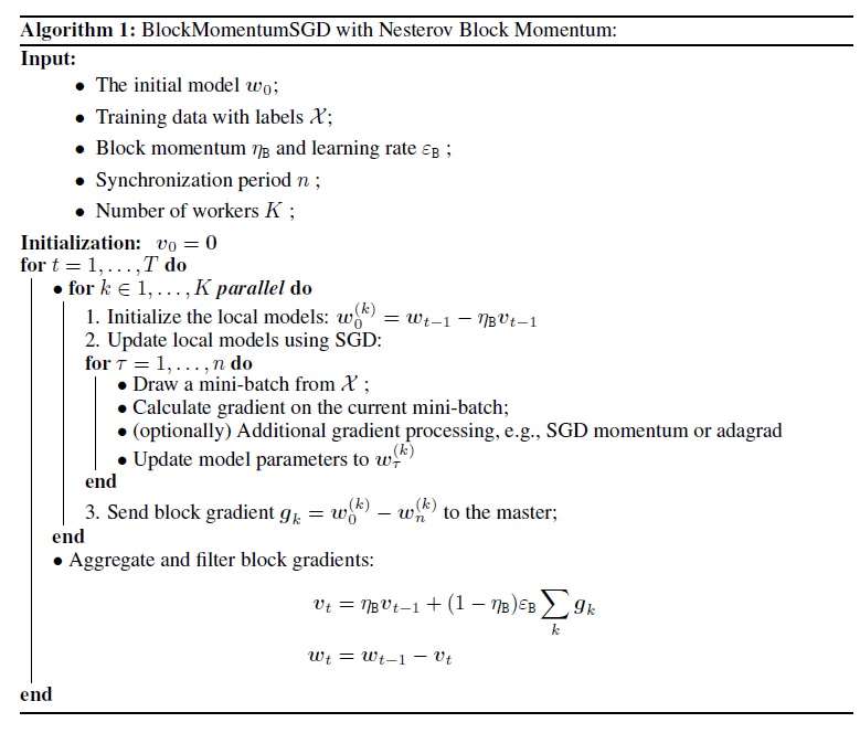
6.1 The Block-Momentum SGD Algorithm

The following figure summarizes the procedure in the Block-Momentum algorithm.

6.2 Configuring Block-Momentum SGD in BrainScript

To use Block-Momentum SGD, it is required to have a sub-block named BlockMomentumSGD in the SGD block with the following options:

1. syncPeriod. This is similar to the syncPeriod in ModelAveragingSGD, which specifies how frequent a model synchronization is performed. The default value for BlockMomentumSGD is 120,000.

2. resetSGDMomentum. This means after every synchronization point, the smoothed gradient used in local SGD will be set as 0. The default value of this variable is true.

3. useNesterovMomentum. This means the Nesterov-style momentum update is applied on the block level. See [2] for more details. The default value of this variable is true.

The block momentum and block learning rate are usually automatically set according to the number of workers used, i.e.,

block_momentum = 1.0 - 1.0/num_of_workers
block_learning_rate = 1.0

Our experience indicates that these settings often yield similar convergence as the standard SGD algorithm up to 64 GPUs, which is the largest experiment we performed. It is also possible to manually specify the these parameters using the following options:

• blockMomentumAsTimeConstant specifies the time constant of the low-pass filter in block-level model update. It is calculated as:

  blockMomentumAsTimeConstant = -syncPeriod / log(block_momentum)
  # or inversely
  block_momentum = exp(-syncPeriod/blockMomentumAsTimeConstant)
  

• blockLearningRate specifies the block learning rate.

Following is an example of Block-Momentum SGD configuration section:

learningRatesPerSample=0.0005
# 0.0005 is the optimal learning rate for single-GPU training.
# Use it for BlockMomentumSGD as well
ParallelTrain = [
    parallelizationMethod = BlockMomentumSGD
    distributedMBReading = true
    syncPerfStats = 5
    BlockMomentumSGD=[
        syncPeriod = 120000
        resetSGDMomentum = true
        useNesterovMomentum = true
    ]
]

6.3 Using Block-Momentum SGD in BrainScript

1. Re-tuning learning parameters

• To achieve similar throughput per worker, it is necessary to increase the number of samples in a minibatch proportional to the number of workers. This can be achieved by adjusting minibatchSize or nbruttsineachrecurrentiter, depending on whether frame-mode randomization is used.

• There is no need to adjust the learning rate (unlike Model-Averaging SGD, see below).

• It is recommended to using Block-Momentum SGD with a warm started model. On our speech recognition tasks, reasonable convergence is achieved when starting from seed models trained on 24 hours (8.6 million samples) to 120 hours (43.2 million samples) data using standard SGD.

2. ASR experiments

We used the Block-Momentum SGD and the Data-Parallel (1-bit) SGD algorithms to train DNNs and LSTMs on a 2600 hours speech-recognition task, and compared word recognition accuracies vs. speed-up factors. The following tables and figures shows the results (*).

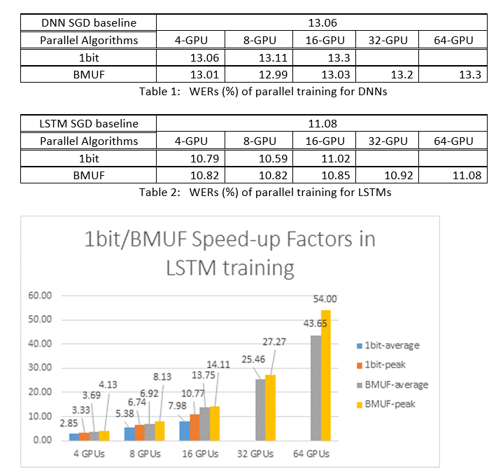
(*): Peak speed-up factor: for 1-bit SGD, measured by the maximum speed-up factor (compared with SGD baseline) achieved in one minibatch; for Block Momentum, measured by the maximum speed-up achieved in one block; Average speed-up factor: the elapsed time in SGD baseline divided by the observed elapsed time. These two metrics are introduced due to the latency in I/O can greatly affect the average speed-up factor measurement, especially when the synchronization is performed at the mini-batch level. At the same time the maximum speed-up factor is relatively robust.

3. Caveats

• It is recommended to set resetSGDMomentum to true; otherwise it often leads to divergence of training criterion. Resetting SGD momentum to 0 after every model synchronization essentially cuts off the contribution from the last minibatches. Therefore, it is recommended not to use a large SGD momentum. For example, for a syncPeriod of 120,000, we observe a significant accuracy loss if the momentum used for SGD is 0.99. Reducing the SGD momentum to 0.9, 0.5 or even disabling it altogether gives similar accuracies as the one can achieved by the standard SGD algorithm.

• Block-Momentum SGD delays and distributes model updates from one block across subsequent blocks. Therefore, it is necessary to make sure that model synchronizations is performed often enough in the training. A quick check is to use blockMomentumAsTimeConstant. It is recommended that the number of unique training samples, N, should satisfy the following equation:

  N >= blockMomentumAsTimeConstant * num_of_workers ~= syncPeriod * num_of_workers^2

The approximation stems from the following facts: (1) Block Momentum is often set as (1-1/num_of_workers); (2) log(1-1/num_of_workers)~=-num_of_workers.

6.4 Using Block-Momentum in Python

To enable Block-Momentum in Python, similarly to the 1-bit SGD, the user needs to create and pass a block momentum distributed learner to the trainer:

from cntk import distributed
...

learner = cntk.learner.momentum_sgd(...)    # create local learner
distributed_learner = cntk.distributed.block_momentum_distributed_learner(learner, block_size=block_size)
...
minibatch_source = MinibatchSource(...) 
...
trainer = Trainer(z, ce, pe, distributed_learner)
...
session = training_session(trainer=trainer, mb_source=minibatch_source, ...)
session.train()
...
distributed.Communicator.finalize()         # must be called to finalize MPI in case of successful distributed training

For a fully functional example please see ConvNet example.

7 Model-Averaging SGD

Model-Averaging SGD is an implementation of the model averaging algorithm detailed in [3,4] without the use of natural gradient. The idea here is to let each worker processes a subset of data, but averaging the model parameters from each worker after a specified period.

Model-Averaging SGD generally converges more slowly and to a worse optimum, compared to 1-bit SGD and Block-Momentum SGD, so it is no longer recommended.

To use Model-Averaging SGD, it is required to have a sub-block named ModelAveragingSGD in the SGD block with the following options:

• syncPeriod specifies the number of samples that each worker need to process before a model averaging is conducted. The default value is 40,000.

7.1 Using Model-Averaging SGD in BrainScript

To make Model-Averaging SGD maximally effective and efficient, users need to tune some hyper-parameters:

• minibatchSize or nbruttsineachrecurrentiter. Suppose n workers are participating in the Model-Averaging SGD configuration, the current distributed reading implementation will load 1/n-th of the minibatch into each worker. Therefore, to make sure each worker produces the same throughput as the standard SGD, it is necessary to enlarge the minibatch size n-fold. For models that are trained using frame-mode randomization, this can be achieved by enlarging minibatchSize by n times; for models are trained using sequence-mode randomization, such as RNNs, some readers require to instead increase nbruttsineachrecurrentiter by n.

• learningRatesPerSample. Our experience indicates that to get similar convergence as the standard SGD, it is necessary to increase the learningRatesPerSample by n times. An explanation can be found in [2]. Since the learning rate is increased, an extra care is needed to make sure the training does not diverge--and this is in fact the main caveat of Model-Averaging SGD. You can use the AutoAdjust settings to reload the previous best model if an increase in training criterion is observed.

• warm start. It is found that Model-Averaging SGD usually converges better if it is started from a seed model which is trained by the standard SGD algorithm (without parallelization). On our speech recognition tasks, reasonable convergence is achieved when starting from seed models trained on 24 hours (8.6 million samples) to 120 hours (43.2 million samples) data using standard SGD.

The following is an example of ModelAveragingSGD configuration section:

learningRatesPerSample = 0.002
# increase the learning rate by 4 times for 4-GPU training.
# learningRatesPerSample = 0.0005
# 0.0005 is the optimal learning rate for single-GPU training.
ParallelTrain = [
    parallelizationMethod = ModelAveragingSGD
    distributedMBReading = true
    syncPerfStats = 20
    ModelAveragingSGD = [
        syncPeriod=40000
    ]
]

7.2 Using Model-Averaging SGD in Python

This is work in progress.

8 Data-Parallel Training with Parameter Server

Parameter server is a widely used framework in distributed machine learning [5][6][7]. The most important benefit it brings is the asynchronous parallel training with many workers. It introduces the parameter server as a distributed model store. Instead of directly leveraging AllReduce primitives to sync parameter updates among workers, parameter server framework provides users the interfaces like "Add" and "Get" to let local workers update and retrieve global parameters from parameter server. In this way, local workers don't need to wait for each other during the training process which saves lots of time especially when the worker number is large.

Furthermore, as parameter servers is a distributed framework that store model parameters, workers can only retrieve those parameters they need during the mini-batch training process, this brings very good flexibility in design distributed training method and also enhances the efficiency when conducting training with sparse model updates. In this release, we will focus on the asynchronous parallel training first, later we will give more introduction on how to leverage parameter server framework for efficient model training with sparse updates.

8.1 Using Data-Parallel ASGD

• To use parameter servers for the Asynchronous SGD (abbr. as ASGD), you should build CNTK with Multiverso supported, Multiverso is a general parameter server framework for distributed machine learning task developed by Microsoft Research Asia team.

• Clone Code: please clone the code under the root folder of CNTK by using:

   git submodule update --init Source/Multiverso

• Linux: please build with --asgd=yes in the configure process.
• Windows: please add CNTK_ENABLE_ASGD to your system environment and set the value to true

• warm start. In some cases, it is better to have the asynchronous model training started from a seed model (which is trained by standard SGD algorithm). In some sense, Asynchronous SGD brings more noise for the training due to the delayed updates from asynchronism among workers. Some models are very sensitive to such noise at the beginning, which might result in diverge of model training. Under such circumstance, a warm start is needed.

8.2 Configuring Data-Parallel ASGD in BrainScript

• To use Data-Parallel ASGD in CNTK, it is required to have a sub-block DataParallelASGD in the SGD block with the following options

• • syncPeriodPerWorkers. It specifies the number of samples that each worker need to process before communicating with the parameter servers. The default value is 256. It's recommended as size of minibatch. It’s obvious that frequent sync up will lead to significant high communication cost. In our test, it’s not necessary to set the value to 1 in most cases.
• • usePipeline. It specifies whether turning on the pipeline of model retrieval and local computation. Turning on the pipeline will significantly increase the overall throughput of training since it will hide some or all of the communication cost. However, sometimes it might slow down the converge rate since more delay will be introduced by adding pipeline. Overall, the clock time will be saved in most cases with pipeline.
• • AdjustLearningRateAtBeginning. According to recently published paper [5], training ASGD is less stable, and it required using much smaller learning rate to avoid occasional explosions of the training loss, therefore the learning process becomes less efficient. However, we found that using lower learning rate is not required for all tasks. And for those tasks sensitive in the beginning, we start the training with small learning rate, and gradually enlarge it at the beginning stage of training process until it reaches the initial learning rate used in normal SGD. In this way, the final accuracy will match SGD while with the speed of ASGD. So we provide this option for ASGD users to leverage this trick. It’s a sub-block in DataParallelASGD with two parameters: adjustCoefficient and adjustNBMiniBatch. The logic is that the learning rate starts from adjustCoefficient of SGD initial learning rate, and increase by adjustCoefficient of SGD initial learning rate every adjustNBMiniBatch mini-batches.

The following is an example of DataParallelASGD configuration section:

   learningRatesPerSample = 0.0005

   ParallelTrain = [
       parallelizationMethod = DataParallelASGD
       distributedMBReading = true
       syncPerfStats = 20
       DataParallelASGD = [
           syncPeriodPerWorker=256
           usePipeline = true
           AdjustLearningRateAtBeginning = [
               adjustCoefficient = 0.2
               adjustNBMiniBatch = 1024
               # Learning rate will be adjusted to original one after ((1 / adjustCoefficient) * adjustNBMiniBatch) samples
               # which is 5120 in this case
           ]
       ]
   ]

8.3 Configuring Data-Parallel ASGD in Python

This is work in progress.

8.4 Experiments

The following figure shows the experiments to test ASGD with CIFAR-10 dataset. The model used in this experiment is a 20-layer ResNet. The asynchronous algorithm reduces the cost on waiting for all worker nodes. ASGD, in this case, is clearly faster than the synchronous algorithms, like MA and SSGD. *In the experiments, all parallel modes synchronize the parameters every iteration (mini-batch update). And for SSGD, we used 32-bit parameter updates. Asynchronous algorithm gains significant advantage in terms of training throughput measured by the sample processing speed, especially when the work node number goes up to 16.

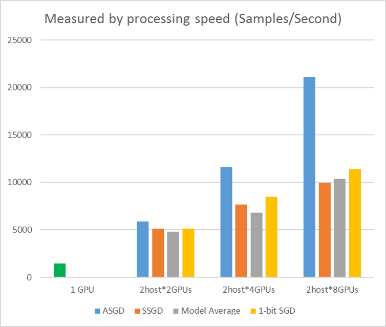Figure 2.4 the speed up for different training methods

References

[1] F. Seide, Hao Fu, Jasha Droppo, Gang Li, and Dong Yu, "1-bit stochastic gradient descent and its application to data-parallel distributed training of speech DNNs," in Proceedings of Interspeech, 2014.

[2] K. Chen and Q. Huo, "Scalable training of deep learning machines by incremental block training with intra-block parallel optimization and blockwise model-update filtering," in Proceedings of ICASSP, 2016.

[3] M. Zinkevich, M. Weimer, L. Li, and A. J. Smola, "Parallelized stochastic gradient descent," in Proceedings of Advances in NIPS, 2010, pp. 2595–2603.

[4] D. Povey, X. Zhang, and S. Khudanpur, "Parallel training of DNNs with natural gradient and parameter averaging," in Proceedings of the International Conference on Learning Representations, 2014.

[5]Chen J, Monga R, Bengio S, et al. Revisiting Distributed Synchronous SGD. ICLR, 2016.

[6]Dean Jeffrey, Greg Corrado, Rajat Monga, Kai Chen, Matthieu Devin, Mark Mao, Andrew Senior et al. Large scale distributed deep networks. In Advances in neural information processing systems, pp. 1223-1231. 2012.

[7]Li Mu, Li Zhou, Zichao Yang, Aaron Li, Fei Xia, David G. Andersen, and Alexander Smola. "Parameter server for distributed machine learning." In Big Learning NIPS Workshop, vol. 6, p. 2. 2013.