Object detection using Fast R-CNN

Table of Contents

• Summary
• Setup
• Run the toy example
• Train on Pascal VOC data
• Train CNTK Fast R-CNN on your own data
• Technical details
• Algorithm details

Summary

This tutorial describes how to use Fast R-CNN in the CNTK Python API. Fast R-CNN using BrainScript and cnkt.exe is described here.

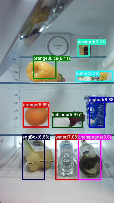
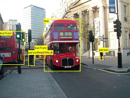
The above are examples images and object annotations for the grocery data set (left) and the Pascal VOC data set (right) used in this tutorial.

Fast R-CNN is an object detection algorithm proposed by Ross Girshick in 2015. The paper is accepted to ICCV 2015, and archived at https://arxiv.org/abs/1504.08083. Fast R-CNN builds on previous work to efficiently classify object proposals using deep convolutional networks. Compared to previous work, Fast R-CNN employs a region of interest pooling scheme that allows to reuse the computations from the convolutional layers.

Setup

To run the code in this example, you need a CNTK Python environment (see here for setup help). Please install the following additional packages in your cntk Python environment

pip install opencv-python easydict pyyaml dlib

Pre-compiled binaries for bounding box regression and non maximum suppression

The folder Examples\Image\Detection\utils\cython_modules contains pre-compiled binaries that are required for running Fast R-CNN. The versions that are currently contained in the repository are Python 3.5 for Windows and Python 3.5, 3.6 for Linux, all 64 bit. If you need a different version you can compile it following the steps described at

• Linux: https://github.com/rbgirshick/py-faster-rcnn
• Windows: https://github.com/MrGF/py-faster-rcnn-windows

Copy the generated cython_bbox and cpu_nms (and/or gpu_nms) binaries from $FRCN_ROOT/lib/utils to $CNTK_ROOT/Examples/Image/Detection/utils/cython_modules.

Example data and baseline model

We use a pre-trained AlexNet model as the basis for Fast-R-CNN training (for VGG or other base models see Using a different base model. Both the example dataset and the pre-trained AlexNet model can be downloaded by running the following Python command from the FastRCNN folder:

python install_data_and_model.py

• Learn how to use a different base model
• Learn how to run Fast R-CNN on Pascal VOC data
• Learn how to run Fast R-CNN on your own data

Run the toy example

To train and evaluate Fast R-CNN run

python run_fast_rcnn.py

The results for training with 2000 ROIs on Grocery using AlexNet as the base model should look similar to these:

AP for          gerkin = 1.0000
AP for          butter = 1.0000
AP for         joghurt = 1.0000
AP for          eggBox = 1.0000
AP for         mustard = 1.0000
AP for       champagne = 1.0000
AP for          orange = 1.0000
AP for           water = 0.5000
AP for         avocado = 1.0000
AP for          tomato = 1.0000
AP for          pepper = 1.0000
AP for         tabasco = 1.0000
AP for           onion = 1.0000
AP for            milk = 1.0000
AP for         ketchup = 0.6667
AP for     orangeJuice = 1.0000
Mean AP = 0.9479

To visualize the predicted bounding boxes and labels on the images open FastRCNN_config.py from the FastRCNN folder and set

__C.VISUALIZE_RESULTS = True

The images will be saved into the FastRCNN/Output/Grocery/ folder if you run python run_fast_rcnn.py.

Train on Pascal VOC

To download the Pascal data and create the annotation files for Pascal in CNTK format run the following scripts:

python Examples/Image/DataSets/Pascal/install_pascalvoc.py
python Examples/Image/DataSets/Pascal/mappings/create_mappings.py

Change the dataset_cfg in the get_configuration() method of run_fast_rcnn.py to

from utils.configs.Pascal_config import cfg as dataset_cfg

Now you're set to train on the Pascal VOC 2007 data using python run_fast_rcnn.py. Beware that training might take a while.

Train on your own data

Prepare a custom dataset

Option #1: Visual Object Tagging Tool (Recommended)

The Visual Object Tagging Tool (VOTT) is a cross platform annotation tool for tagging video and image assets.

VOTT provides the following features:

• Computer-assisted tagging and tracking of objects in videos using the Camshift tracking algorithm.
• Exporting tags and assets to CNTK Fast-RCNN format for training an object detection model.
• Running and validating a trained CNTK object detection model on new videos to generate stronger models.

How to annotate with VOTT:

1. Download the latest Release
2. Follow the Readme to run a tagging job
3. After tagging Export tags to the dataset directory

Option #2: Using Annotation Scripts

To train a CNTK Fast R-CNN model on your own data set we provide two scripts to annotate rectangular regions on images and assign labels to these regions. The scripts will store the annotations in the correct format as required by the first step of running Fast R-CNN (A1_GenerateInputROIs.py). First, store your images in the following folder structure

• <your_image_folder>/negative - images used for training that don't contain any objects
• <your_image_folder>/positive - images used for training that do contain objects
• <your_image_folder>/testImages - images used for testing that do contain objects

For the negative images you do not need to create any annotations. For the other two folders use the provided scripts:

• Run C1_DrawBboxesOnImages.py to draw bounding boxes on the images.
  • In the script set imgDir = <your_image_folder> (/positive or /testImages) before running.
  • Add annotations using the mouse cursor. Once all objects in an image are annotated, pressing key 'n' writes the .bboxes.txt file and then proceeds to the next image, 'u' undoes (i.e. removes) the last rectangle, and 'q' quits the annotation tool.
• Run C2_AssignLabelsToBboxes.py to assign labels to the bounding boxes.
  • In the script set imgDir = <your_image_folder> (/positive or /testImages) before running...
  • ... and adapt the classes in the script to reflect your object categories, for example classes = ("dog", "cat", "octopus").
  • The script loads these manually annotated rectangles for each image, displays them one-by-one, and asks the user to provide the object class by clicking on the respective button to the left of the window. Ground truth annotations marked as either "undecided" or "exclude" are fully excluded from further processing.

Train on custom dataset

After storing your images in the described folder structure and annotating them please run

python Examples/Image/Detection/utils/annotations/annotations_helper.py

after changing the folder in that script to your data folder. Finally, create a MyDataSet_config.py in the utils\configs folder following the existing examples:

__C.CNTK.DATASET == "YourDataSet":
__C.CNTK.MAP_FILE_PATH = "../../DataSets/YourDataSet"
__C.CNTK.CLASS_MAP_FILE = "class_map.txt"
__C.CNTK.TRAIN_MAP_FILE = "train_img_file.txt"
__C.CNTK.TEST_MAP_FILE = "test_img_file.txt"
__C.CNTK.TRAIN_ROI_FILE = "train_roi_file.txt"
__C.CNTK.TEST_ROI_FILE = "test_roi_file.txt"
__C.CNTK.NUM_TRAIN_IMAGES = 500
__C.CNTK.NUM_TEST_IMAGES = 200
__C.CNTK.PROPOSAL_LAYER_SCALES = [8, 16, 32]

Note that __C.CNTK.PROPOSAL_LAYER_SCALES is not used for Fast R-CNN, only for Faster R-CNN.

To train and evaluate Fast R-CNN on your data change the dataset_cfg in the get_configuration() method of run_fast_rcnn.py to

from utils.configs.MyDataSet_config import cfg as dataset_cfg

and run python run_fast_rcnn.py.

Technical details

The Fast R-CNN algorithm is explained in the Algorithm details section together with a high level overview of how it is implemented in the CNTK Python API. This section focuses on configuring Fast R-CNN and how to you use different base models.

Parameters

The parameters are grouped into three parts:

• Detector parameters (see FastRCNN/FastRCNN_config.py)
• Data set parameters (see for example utils/configs/Grocery_config.py)
• Base model parameters (see for example utils/configs/AlexNet_config.py)

The three parts are loaded and merged in the get_configuration() method in run_fast_rcnn.py. In this section we'll cover the detector parameters. Data set parameters are described here, base model parameters here. In the following we go through the most important parameters in FastRCNN_config.py. All parameters are also commented in the file. The configuration uses the EasyDict package that allows easy access to nested dictionaries.

# Number of regions of interest [ROIs] proposals
__C.NUM_ROI_PROPOSALS = 200 # use 2000 or more for good results
# the minimum IoU (overlap) of a proposal to qualify for training regression targets
__C.BBOX_THRESH = 0.5

# Maximum number of ground truth annotations per image
__C.INPUT_ROIS_PER_IMAGE = 50
__C.IMAGE_WIDTH = 850
__C.IMAGE_HEIGHT = 850

# Use horizontally-flipped images during training?
__C.TRAIN.USE_FLIPPED = True
# If set to 'True' conv layers weights from the base model will be trained, too
__C.TRAIN_CONV_LAYERS = True

The ROI proposals are computed on the fly in the first epoch using the selective search implementation from the dlib package. The number of proposals that are generated is controlled by the __C.NUM_ROI_PROPOSALS parameter. We recommend to use around 2000 proposals. The regression head is only trained on those ROIs that have an overlap (IoU) with a ground truth box of at least __C.BBOX_THRESH.

__C.INPUT_ROIS_PER_IMAGE specifies the maximum number of ground truth annotations per image. CNTK currently requires to set a maximum number. If there are fewer annotations they will be padded internally. __C.IMAGE_WIDTH and __C.IMAGE_HEIGHT are the dimensions that are used to resize and pad the input images.

__C.TRAIN.USE_FLIPPED = True will augment the training data by flipping all images every other epoch, i.e. the first epoch has all regular images, the second has all images flipped, and so forth. __C.TRAIN_CONV_LAYERS determines whether the convolutional layers, from input to the convolutional feature map, will be trained or fixed. Fixing the conv layer weights means that the weights from the base model are taken and not modified during training. (You can also specify how many conv layers you want to train, see section Using a different base model).

# NMS threshold used to discard overlapping predicted bounding boxes
__C.RESULTS_NMS_THRESHOLD = 0.5

# If set to True the following two parameters need to point to the corresponding files that contain the proposals:
# __C.DATA.TRAIN_PRECOMPUTED_PROPOSALS_FILE
# __C.DATA.TEST_PRECOMPUTED_PROPOSALS_FILE
__C.USE_PRECOMPUTED_PROPOSALS = False

__C.RESULTS_NMS_THRESHOLD is the NMS threshold used to discard overlapping predicted bounding boxes in evaluation. A lower threshold yields fewer removals and hence more predicted bounding boxes in the final output. If you set __C.USE_PRECOMPUTED_PROPOSALS = True the reader will read precomputed ROIs from text files. This is for example used for training on Pascal VOC data. The file names __C.DATA.TRAIN_PRECOMPUTED_PROPOSALS_FILE and __C.DATA.TEST_PRECOMPUTED_PROPOSALS_FILE are specified in Examples/Image/Detection/utils/configs/Pascal_config.py.

# The basic segmentation is performed kvals.size() times. The k parameter is set (from, to, step_size)
__C.roi_ss_kvals = (10, 500, 5)
# When doing the basic segmentations prior to any box merging, all
# rectangles that have an area < min_size are discarded. Therefore, all outputs and
# subsequent merged rectangles are built out of rectangles that contain at
# least min_size pixels. Note that setting min_size to a smaller value than
# you might otherwise be interested in using can be useful since it allows a
# larger number of possible merged boxes to be created
__C.roi_ss_min_size = 9
# There are max_merging_iterations rounds of neighboring blob merging.
# Therefore, this parameter has some effect on the number of output rectangles
# you get, with larger values of the parameter giving more output rectangles.
# Hint: set __C.CNTK.DEBUG_OUTPUT=True to see the number of ROIs from selective search
__C.roi_ss_mm_iterations = 30
# image size used for ROI generation
__C.roi_ss_img_size = 200

The above parameters are configuring dlib's selective search. For details see the dlib homepage. The following additional parameters are used to filter generated ROIs w.r.t. minimum and maximum side length, area and aspect ratio.

# minimum relative width/height of an ROI
__C.roi_min_side_rel = 0.01
# maximum relative width/height of an ROI
__C.roi_max_side_rel = 1.0
# minimum relative area of an ROI
__C.roi_min_area_rel = 0.0001
# maximum relative area of an ROI
__C.roi_max_area_rel = 0.9
# maximum aspect ratio of an ROI vertically and horizontally
__C.roi_max_aspect_ratio = 4.0
# aspect ratios of ROIs for uniform grid ROIs
__C.roi_grid_aspect_ratios = [1.0, 2.0, 0.5]

If selective search returns more ROIs than requested they are sampled randomly. If fewer ROIs are return additional ROIs are generated on a regular grid using the specified __C.roi_grid_aspect_ratios.

Using a different base model

To use a different base model you need to choose a different model configuration in the get_configuration() method of run_fast_rcnn.py. Two models are supported right away:

    # for VGG16 base model use:         from utils.configs.VGG16_config import cfg as network_cfg
    # for AlexNet base model use:       from utils.configs.AlexNet_config import cfg as network_cfg

To download the VGG16 model please use the download script in <cntkroot>/PretrainedModels:

    python download_model.py VGG16_ImageNet_Caffe

If you want to use another different base model you need to copy, for example, the configuration file utils/configs/VGG16_config.py and modify it according to your base model:

# model config
__C.MODEL.BASE_MODEL = "VGG16"
__C.MODEL.BASE_MODEL_FILE = "VGG16_ImageNet_Caffe.model"
__C.MODEL.IMG_PAD_COLOR = [103, 116, 123]
__C.MODEL.FEATURE_NODE_NAME = "data"
__C.MODEL.LAST_CONV_NODE_NAME = "relu5_3"
__C.MODEL.START_TRAIN_CONV_NODE_NAME = "pool2" # __C.MODEL.FEATURE_NODE_NAME
__C.MODEL.POOL_NODE_NAME = "pool5"
__C.MODEL.LAST_HIDDEN_NODE_NAME = "drop7"
__C.MODEL.FEATURE_STRIDE = 16
__C.MODEL.RPN_NUM_CHANNELS = 512
__C.MODEL.ROI_DIM = 7

To investigate the node names of your base model you can use the plot() method from cntk.logging.graph. Please note that ResNet models are currently not supported since roi pooling in CNTK does not yet support roi average pooling.

Algorithm details

Fast R-CNN

R-CNNs for Object Detection were first presented in 2014 by Ross Girshick et al., and were shown to outperform previous state-of-the-art approaches on one of the major object recognition challenges in the field: Pascal VOC. Since then, two follow-up papers were published which contain significant speed improvements: Fast R-CNN and Faster R-CNN.

The basic idea of R-CNN is to take a deep Neural Network which was originally trained for image classification using millions of annotated images and modify it for the purpose of object detection. The basic idea from the first R-CNN paper is illustrated in the Figure below (taken from the paper): (1) Given an input image, (2) in a first step, a large number region proposals are generated. (3) These region proposals, or Regions-of-Interests (ROIs), are then each independently sent through the network which outputs a vector of e.g. 4096 floating point values for each ROI. Finally, (4) a classifier is learned which takes the 4096 float ROI representation as input and outputs a label and confidence to each ROI.

While this approach works well in terms of accuracy, it is very costly to compute since the Neural Network has to be evaluated for each ROI. Fast R-CNN addresses this drawback by only evaluating most of the network (to be specific: the convolution layers) a single time per image. According to the authors, this leads to a 213 times speed-up during testing and a 9x speed-up during training without loss of accuracy. This is achieved by using an ROI pooling layer which projects the ROI onto the convolutional feature map and performs max pooling to generate the desired output size that the following layer is expecting. In the AlexNet example used in this tutorial the ROI pooling layer is put between the last convolutional layer and the first fully connected layer. In the CNTK Python API code shown below this is realized by cloning two parts of the network, the conv_layers and the fc_layers. The input image is then first normalized, pushed through the conv_layers, the roipooling layer and the fc_layers and finally the prediction and regression heads are added that predict the class label and the regression coefficients per candidate ROI respectively.

def create_fast_rcnn_model(features, roi_proposals, label_targets, bbox_targets, bbox_inside_weights, cfg):
    # Load the pre-trained classification net and clone layers
    base_model = load_model(cfg['BASE_MODEL_PATH'])
    conv_layers = clone_conv_layers(base_model, cfg)
    fc_layers = clone_model(base_model, [cfg["MODEL"].POOL_NODE_NAME], [cfg["MODEL"].LAST_HIDDEN_NODE_NAME], clone_method=CloneMethod.clone)

    # Normalization and conv layers
    feat_norm = features - Constant([[[v]] for v in cfg["MODEL"].IMG_PAD_COLOR])
    conv_out = conv_layers(feat_norm)

    # Fast RCNN and losses
    cls_score, bbox_pred = create_fast_rcnn_predictor(conv_out, roi_proposals, fc_layers, cfg)
    detection_losses = create_detection_losses(...)
    pred_error = classification_error(cls_score, label_targets, axis=1)

    return detection_losses, pred_error

def create_fast_rcnn_predictor(conv_out, rois, fc_layers, cfg):
    # RCNN
    roi_out = roipooling(conv_out, rois, cntk.MAX_POOLING, (6, 6), spatial_scale=1/16.0)
    fc_out = fc_layers(roi_out)

    # prediction head
    cls_score = plus(times(fc_out, W_pred), b_pred, name='cls_score')

    # regression head
    bbox_pred = plus(times(fc_out, W_regr), b_regr, name='bbox_regr')

    return cls_score, bbox_pred

The original Caffe implementation used in the R-CNN papers can be found at GitHub: RCNN, Fast R-CNN, and Faster R-CNN.

SVM vs NN training

Patrick Buehler provides instructions on how to train an SVM on the CNTK Fast R-CNN output (using the 4096 features from the last fully connected layer) as well as a discussion on pros and cons here.

Selective Search

Selective Search is a method for finding a large set of possible object locations in an image, independent of the class of the actual object. It works by clustering image pixels into segments, and then performing hierarchical clustering to combine segments from the same object into object proposals.

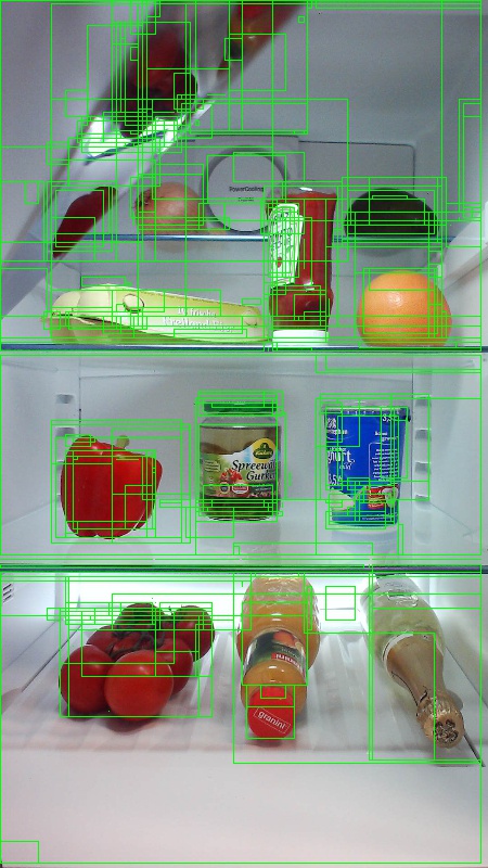
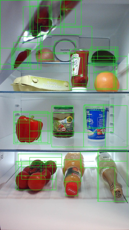
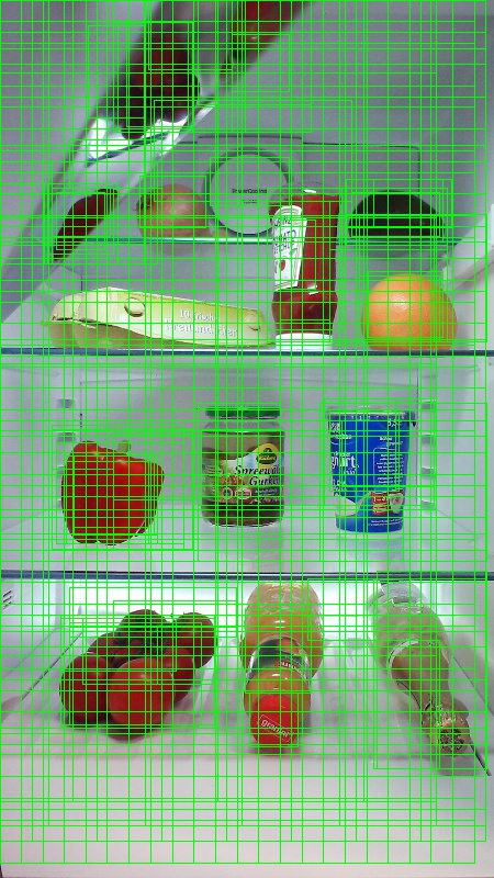
To complement the detected ROIs from Selective Search, we add ROIs that uniform cover the image at different scales and aspect ratios. The image on the left shows an example output of Selective Search, where each possible object location is visualized by a green rectangle. ROIs that are too small, too big, etc. are discarded (middle) and finally ROIs that uniformly cover the image are added (right). These rectangles are then used as Regions-of-Interests (ROIs) in the R-CNN pipeline.

The goal of ROI generation is to find a small set of ROIs which however tightly cover as many objects in the image as possible. This computation has to be sufficiently quick, while at the same time finding object locations at different scales and aspect ratios. Selective Search was shown to perform well for this task, with good accuracy to speed trade-offs.

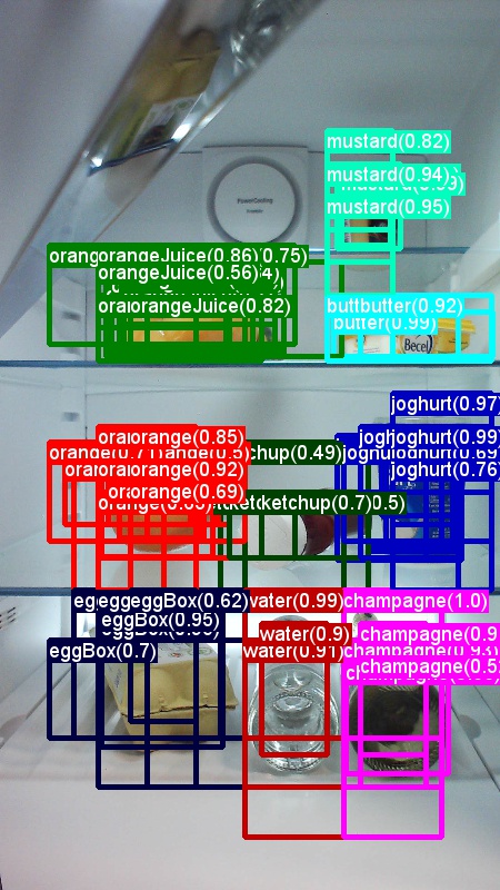
NMS (Non Maximum Suppression)

Object detection methods often output multiple detections which fully or partly cover the same object in an image. These ROIs need to be merged to be able to count objects and obtain their exact locations in the image. This is traditionally done using a technique called Non Maximum Suppression (NMS). The version of NMS we use (and which was also used in the R-CNN publications) does not merge ROIs but instead tries to identify which ROIs best cover the real locations of an object and discards all other ROIs. This is implemented by iteratively selecting the ROI with highest confidence and removing all other ROIs which significantly overlap this ROI and are classified to be of the same class. The threshold for the overlap can be set in PARAMETERS.py (details).

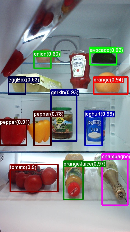
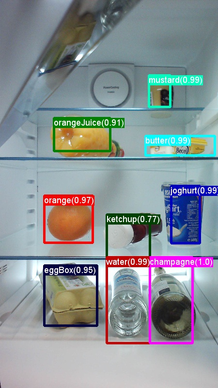
Detection results before (left) and after (right) Non Maximum Suppression:

mAP (mean Average Precision)

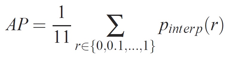
Once trained, the quality of the model can be measured using different criteria, such as precision, recall, accuracy, area-under-curve, etc. A common metric which is used for the Pascal VOC object recognition challenge is to measure the Average Precision (AP) for each class. The following description of Average Precision is taken from Everingham et. al. The mean Average Precision (mAP) is computed by taking the average over the APs of all classes.

For a given task and class, the precision/recall curve is computed from a method’s ranked output. Recall is defined as the proportion of all positive examples ranked above a given rank. Precision is the proportion of all examples above that rank which are from the positive class. The AP summarizes the shape of the precision/recall curve, and is defined as the mean precision at a set of eleven equally spaced recall levels [0,0.1, . . . ,1]:

The precision at each recall level r is interpolated by taking the maximum precision measured for a method for which the corresponding recall exceeds r:

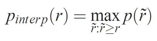
where p(˜r) is the measured precision at recall ˜r. The intention in interpolating the precision/recall curve in this way is to reduce the impact of the “wiggles” in the precision/recall curve, caused by small variations in the ranking of examples. It should be noted that to obtain a high score, a method must have precision at all levels of recall – this penalizes methods which retrieve only a subset of examples with high precision (e.g. side views of cars).