Note
Access to this page requires authorization. You can try signing in or changing directories.
Access to this page requires authorization. You can try changing directories.
CNTK provides a simple way to visualize the underlying computational graph of a model using Graphviz, an open-source graph visualization software.
To illustrate a use case, let's first build a simple convolutional network using the CNTK Layers library.
import cntk as C

def create_model(x, num_classes):
  with C.layers.default_options(init=C.glorot_uniform(), activation=C.relu):
    model = C.layers.Sequential([
      C.layers.For(range(3), lambda i: [
        C.layers.Convolution((5,5), [32,32,64][i], pad=True, name=['conv1', 'conv2', 'conv3'][i]),
        C.layers.MaxPooling((3,3), strides=(2,2), name=['pool1', 'pool2', 'pool3'][i])
        ]),
      C.layers.Dense(64, name='fc1'),
      C.layers.Dense(num_classes, activation=None, name='classify')
    ])
  return model(x)
Now assuming we are training on the CIFAR-10 dataset, which consists of 32x32 images in 10 classes, we can assign the input shape correspondingly. Refer to the CNTK 201A tutorial for instructions on downloading and preparing the CIFAR-10 dataset for use in CNTK.
input_var = C.input_variable((3,32,32))
z = create_model(input_var)
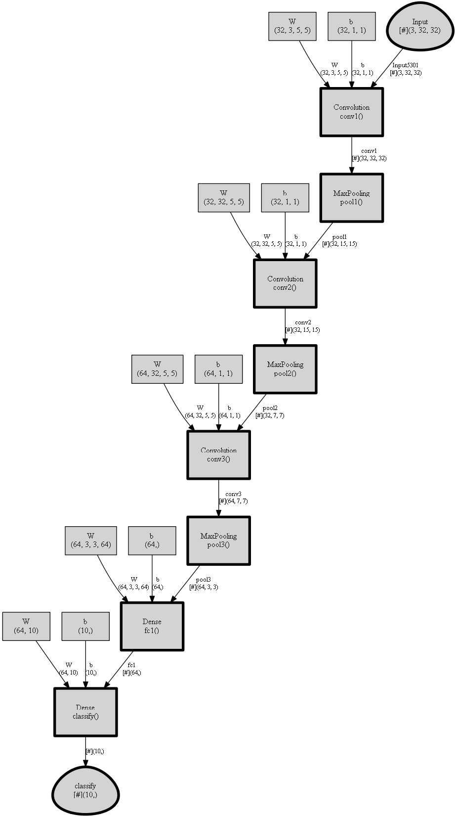
To get the underlying description of the computational graph, CNTK provides a plot function in the cntk.logging.graph module.
The plot(root, filename=None) function returns a network description of the graph starting at the root node provided. In addition, if filename is specified, the method outputs a DOT, PNG, PDF or SVG file (corresponding to the filename suffix).
In order to output the DOT output, you will need to install pydot-ng (pip install pydot_ng). And if you would like PNG, PDF or SVG output, you will need Graphviz in addition to pydot-ng.
Once you've installed Graphviz, ensure that the Graphviz binaries are in your PATH environment variable.
import pydot_ng

graph_description = C.logging.graph.plot(z, "graph.png")
print(graph_description)
Convolution(Parameter5302, Parameter5303, Input5301) -> Block6011_Output_0;

MaxPooling(Block6011_Output_0) -> Block6023_Output_0;

Convolution(Parameter5332, Parameter5333, Block6023_Output_0) -> Block6039_Output_0;

MaxPooling(Block6039_Output_0) -> Block6051_Output_0;

Convolution(Parameter5362, Parameter5363, Block6051_Output_0) -> Block6067_Output_0;

MaxPooling(Block6067_Output_0) -> Block6079_Output_0;

Dense(Parameter5710, Parameter5711, Block6079_Output_0) -> Block6095_Output_0;

Dense(Parameter5730, Parameter5731, Block6095_Output_0) -> Block6110_Output_0;
If you are using a Jupyter Notebook, you can display the graph visualization output inline:
from IPython.display import Image

display(Image(filename="graph.png"))
For a more detailed example of visualization using logging.graph.plot, refer to the How to debug manual.