Note
Access to this page requires authorization. You can try signing in or changing directories.
Access to this page requires authorization. You can try changing directories.
The conditional formatting feature in PowerTable sheets helps highlight specific data based on defined conditions. Use conditional formatting to emphasize records with text styles, borders, icons, font colors, or background colors. This formatting makes it easier to identify trends, exceptions, outliers, and other important data points.
PowerTable automatically applies conditional formatting rules to table data when the data meets the specified conditions. You can create, manage, edit, and remove rules to customize how data appears and improve the readability of your sheets.
Common use cases for conditional formatting include:
- Highlighting values that exceed or fall below a target threshold.
- Identifying records that require attention or follow-up.
- Visualizing performance metrics using color indicators.
- Emphasizing specific text values or statuses.
- Drawing attention to missing, duplicate, or exceptional data.
By using conditional formatting, you can quickly interpret large datasets and focus on the information that matters most.
In this article, you learn how to apply conditional formatting by configuring and managing rules.
Create a conditional formatting rule
To create a conditional formatting rule:
Go to the Format tab and select Format Rules > Create Rule.
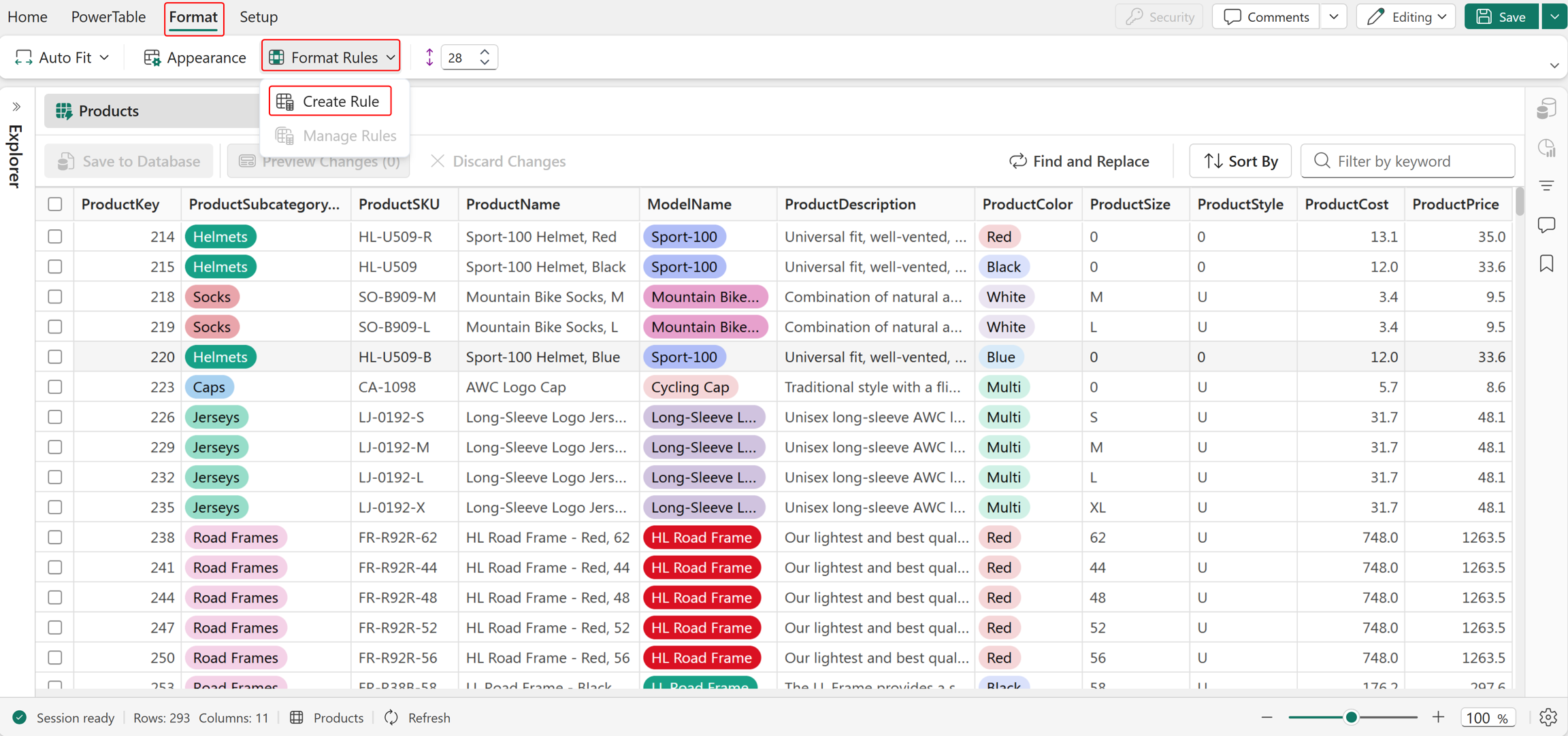
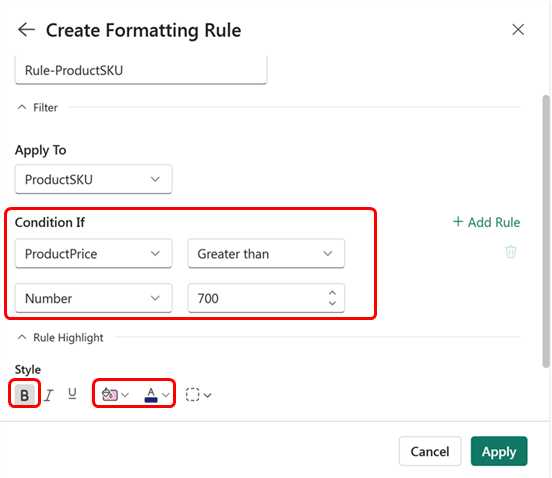
A side panel opens, as the following image shows.
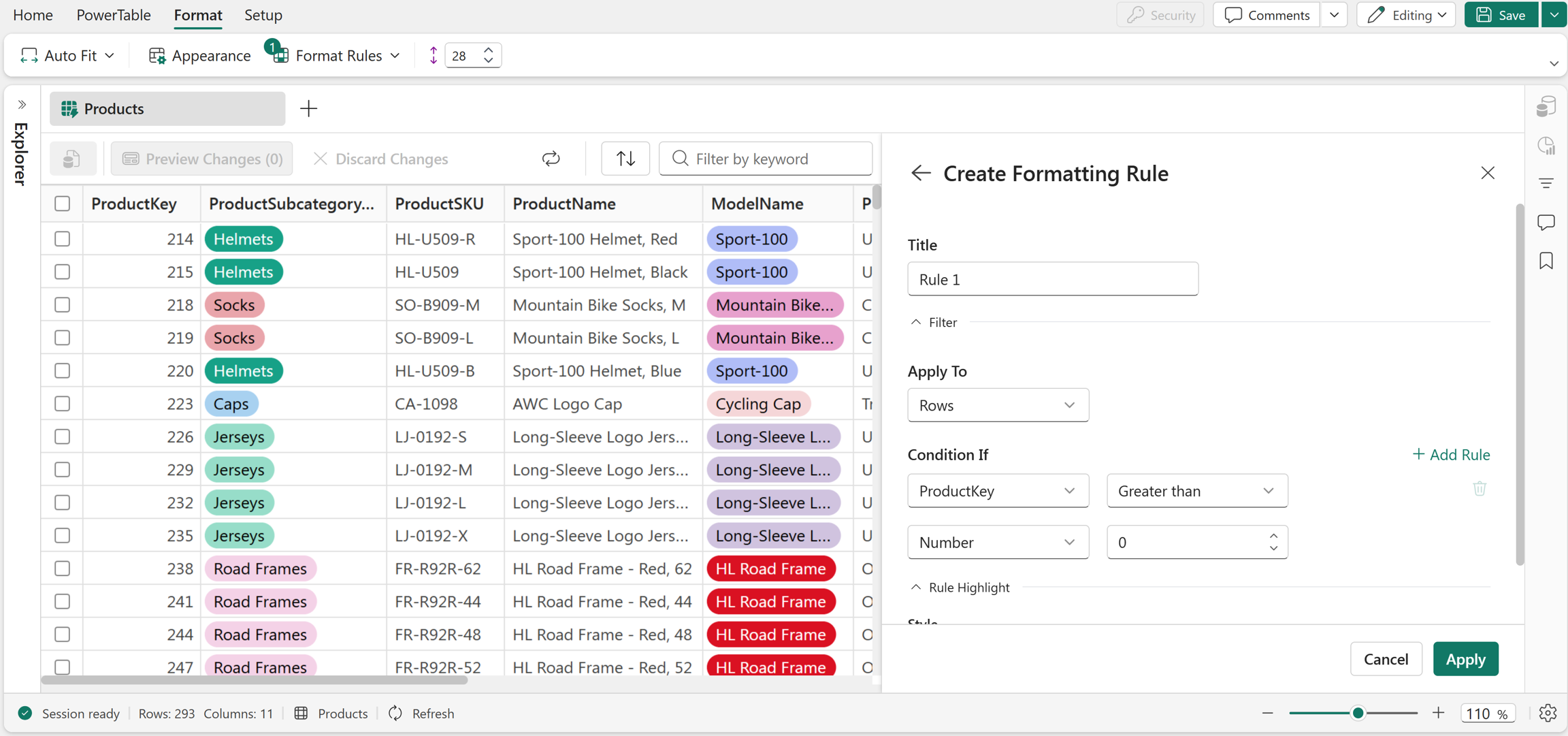
In Title, enter a name for the rule.
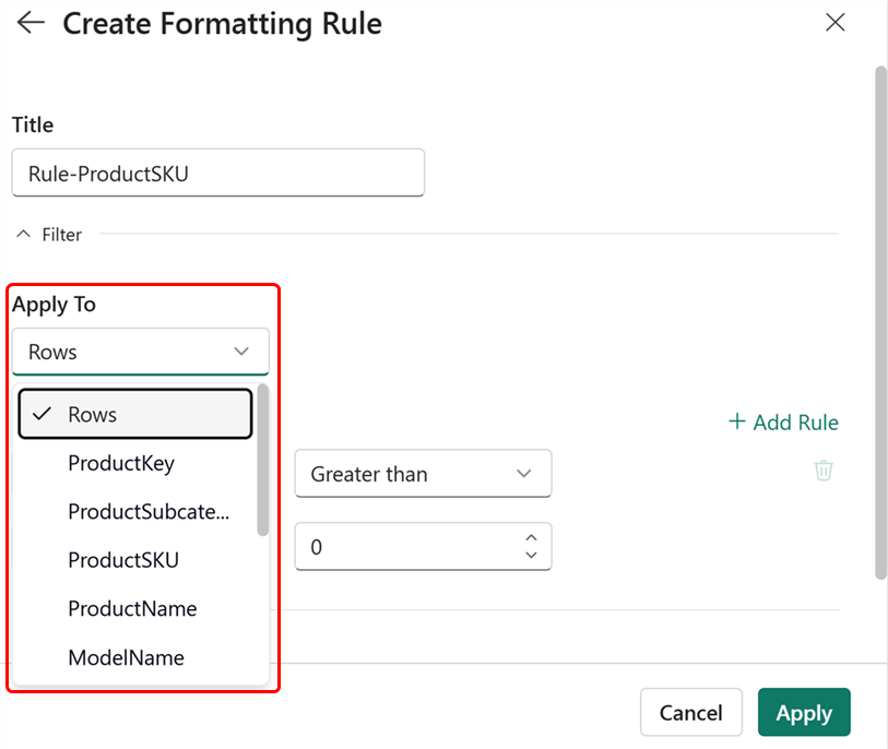
In Apply To, select the column or rows to format.
Use Conditions to define the criteria for the rule. The available operators and comparison options vary based on the selected column type.
In Style, configure the formatting to apply when the condition is true. You can customize font color, font style, borders, background color, or specific icons.
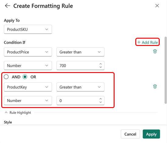
Select Add Rule to add more conditions. You can combine multiple conditions by using AND or OR operators.
Select Apply to save and apply the rule. To discard the changes, select Cancel.
Apply to column
When you select a column, formatting applies only to the records in the selected column that meet the specified condition. For example:
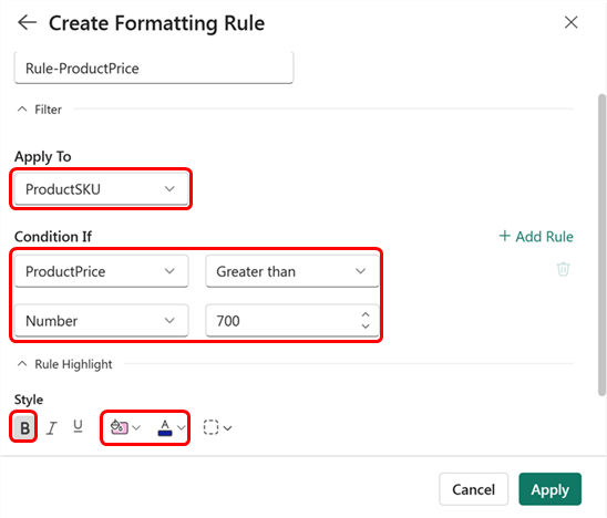
Select the ProductSKU column in the Apply To dropdown.
Configure the condition as ProductPrice Greater than 700 in the Condition If section.
Configure the formatting style by applying bold text, the required font color, and background color.
Optionally, use the Add Prefix/Suffix option to add text or an icon before or after the cell value by customizing the icon type, icon color, text, and position.
Note
The Add Prefix/Suffix option is available only when you select a column in the Apply To field.
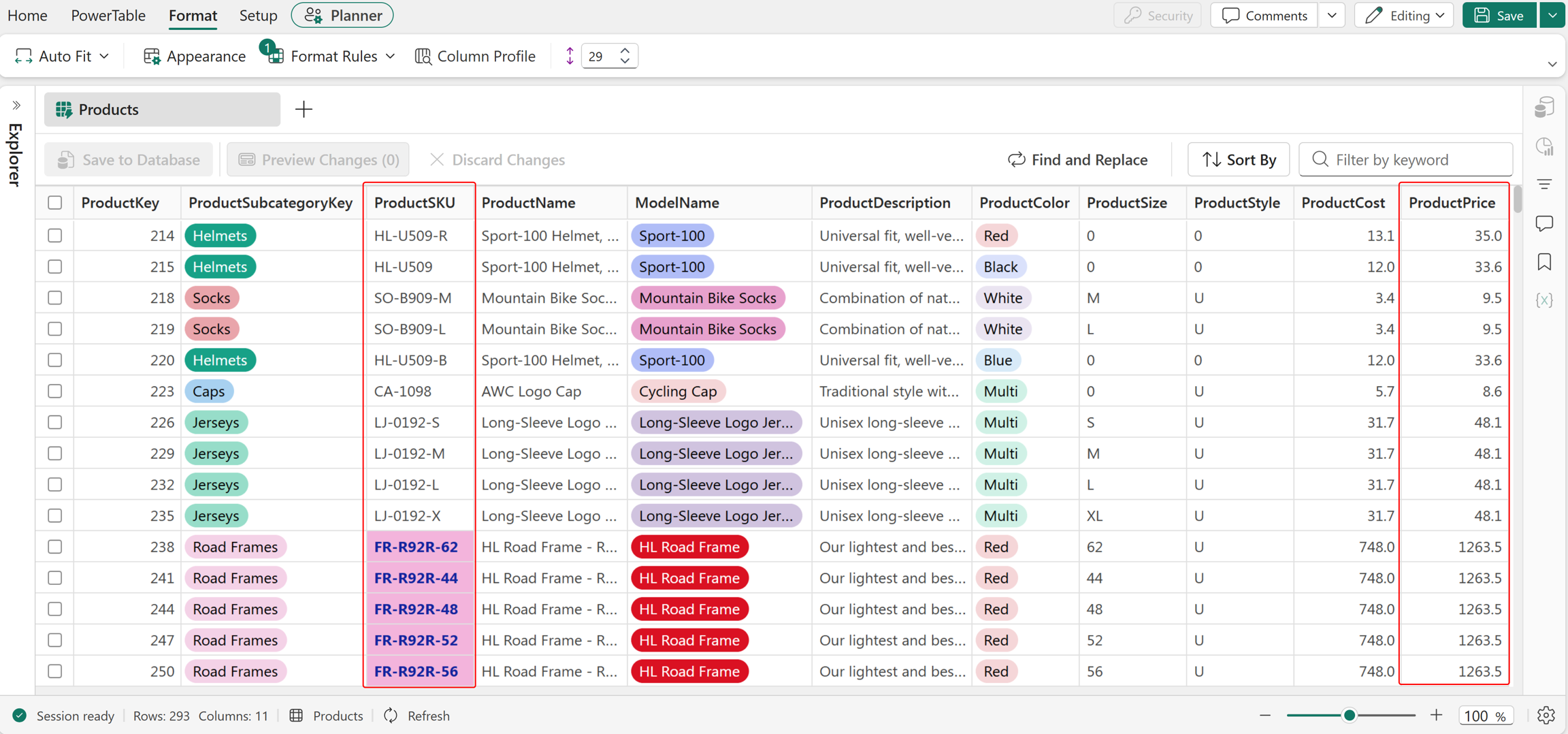
The following image shows the formatted records in the ProductSKU column that meet the configured condition.
Apply to rows
To apply formatting to all columns in rows that meet the specified condition, select Rows in the Apply To dropdown. For example:
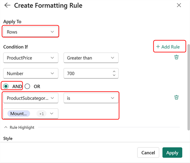
Consider formatting rows that contain products with a price greater than 700 and a subcategory of mountain bikes or road bikes.
To format all columns in the rows that meet the specified conditions, select Rows in the Apply To dropdown.
In the Condition If section, set the first condition to ProductPrice Greater than 700.
Select Add Rule to add the second condition.
Set the second condition to ProductSubcategoryKey is Mountain Bikes or Road Bikes.
Select AND to combine the two conditions.
Select Apply.
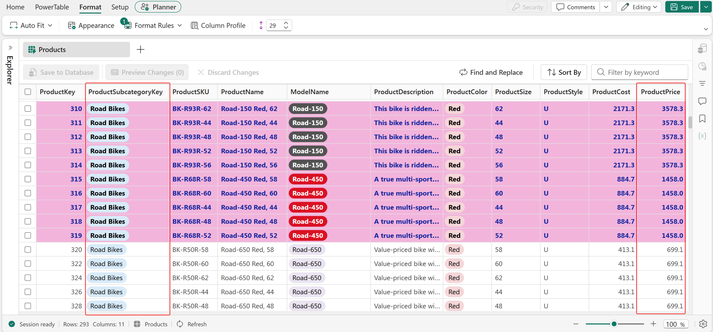
All columns in rows that meet the configured conditions are formatted as shown in the following image.
Manage conditional formatting rules
Use Manage Rules to view, edit, duplicate, disable, or delete existing conditional formatting rules.
To manage rules:
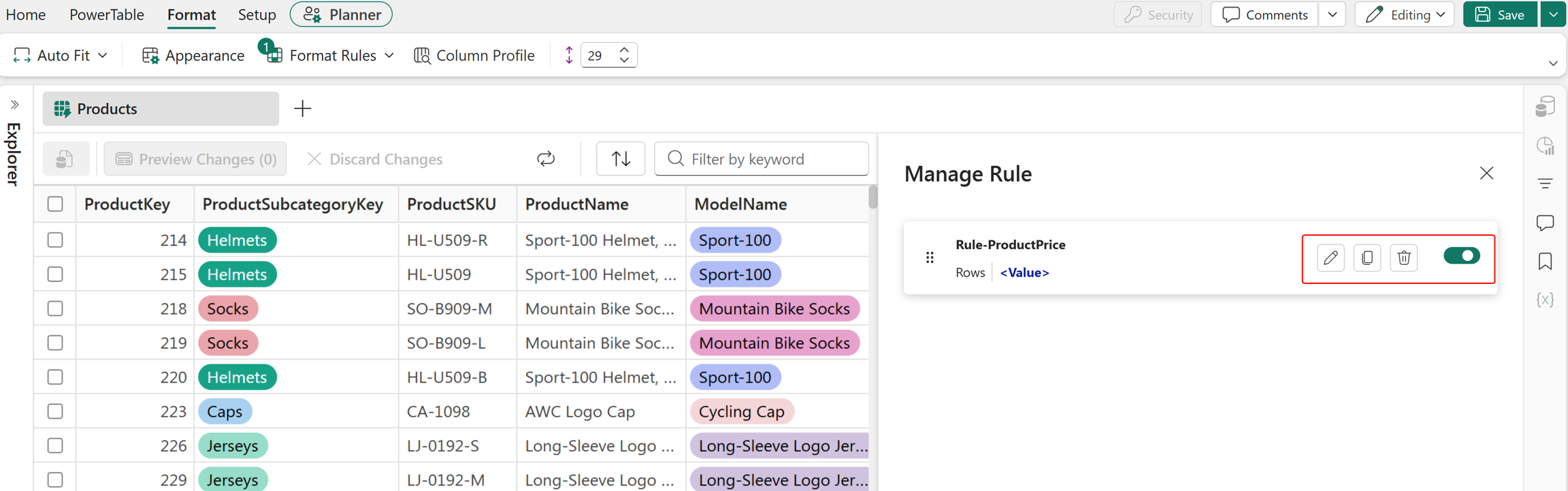
Select Format Rules > Manage Rules. A side panel opens and shows all configured rules.
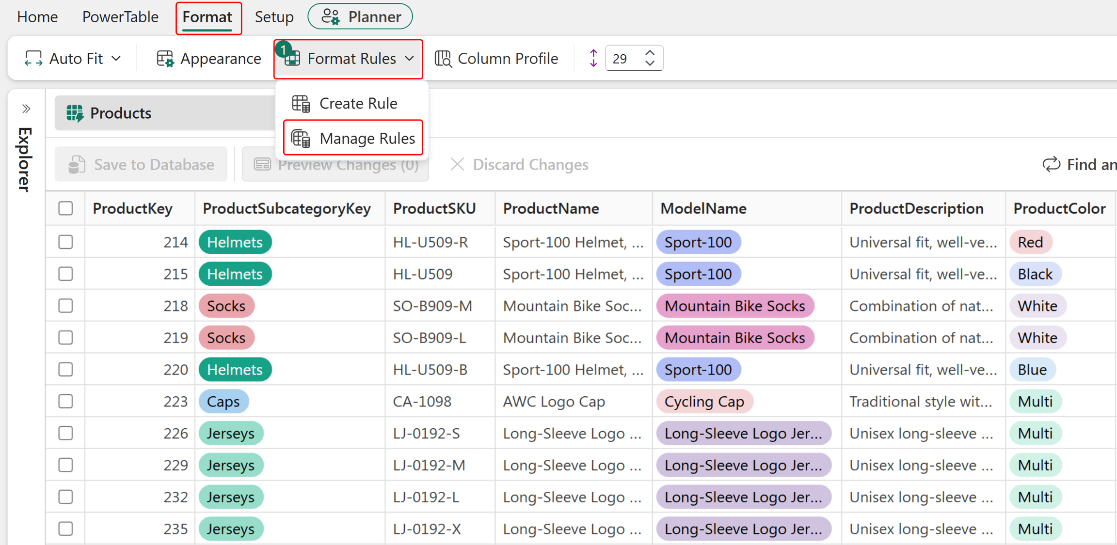
Use the available actions for a rule to edit, duplicate, delete, enable, or disable it.