Note
Access to this page requires authorization. You can try signing in or changing directories.
Access to this page requires authorization. You can try changing directories.
Important
This content is being retired and may not be updated in the future. The support for Machine Learning Server will end on July 1, 2022. For more information, see What's happening to Machine Learning Server?
A crucial step in many analyses is transforming the data into a form best suited for the chosen analysis. For example, to reduce variations in scale between variables, you might take a log or a power of the original variable before fitting the dataset to a linear model. Additionally, transforming data minimizes passes through the data, which is more efficient.
In RevoScaleR, you can perform data transformations in virtually all of its functions, from rxImport to rxDataStep, as well as the analysis functions rxSummary, rxLinMod, rxLogit, rxGlm, rxCrossTabs, rxCube, rxCovCor, and rxKmeans.
In all cases, the basic approach for data transforms is the same. The heart of the RevoScaleR data step is a list of transforms, each of which specifies an R expression to be evaluated. The data step typically is an assignment that either creates a new variable or modifies an existing variable from the original data set.
This article uses examples to illustrate common data manipulation tasks. For more background, see Data Transformations.
Subset data by row or variable
A common use of rxDataStep is to create a new data set with a subset of rows and variables. The following simple example uses a data frame as the input data set.
The call to rxDataStep uses the rowSelection argument to select only the rows where the variable y is greater than .5, and the varsToKeep argument to keeps only the variables y and z. The rowSelection argument is an R expression that evaluates to TRUE if the observation should be kept. The varsToKeep argument contains a list of variable names to read in from the original data set. Because no outFile is specified, a data frame is returned.
# Create a data frame
set.seed(59)
myData <- data.frame(
x = rnorm(100),
y = runif(100),
z = rep(1:20, times = 5))

# Subset observations and variables
myNewData <- rxDataStep( inData = myData,
	rowSelection = y > .5,
	varsToKeep = c("y", "z"))

# Get information about the new data frame
rxGetInfo(data = myNewData, getVarInfo = TRUE)
You should see the following results:
Data frame: myNewData
Number of observations: 52
Number of variables: 2
Variable information:
Var 1: y, Type: numeric, Low/High: (0.5516, 0.9941)
Var 2: z, Type: integer, Low/High: (1, 20)
Subsetting is particularly useful if your original data set contains millions of rows or hundreds of thousands of variables. As a smaller example, the CensusWorkers.xdf sample data file has six variables and 351,121 rows.
To create a subset containing only workers who have worked less than 30 weeks in the year and five variables, we can again use rxDataStep with the rowSelection and varsToKeep arguments. Since the resulting data set will clearly fit in memory, we omit the outFile argument and assign the result of the data step, then use rxGetInfo to see our results as usual:
readPath <- rxGetOption("sampleDataDir")
censusWorkers <- file.path(readPath, "CensusWorkers.xdf")
partWorkers <- rxDataStep(inData = censusWorkers, rowSelection = wkswork1 < 30,
				varsToKeep = c("age", "sex", "wkswork1", "incwage", "perwt"))
rxGetInfo(partWorkers, getVarInfo = TRUE)
The result is a data set with 14,317 rows:
	Data frame: partWorkers
	Number of observations: 14317
	Number of variables: 5
	Variable information:
	Var 1: age, Age
	       Type: integer, Low/High: (20, 65)
	Var 2: sex, Sex
	       2 factor levels: Male Female
	Var 3: wkswork1, Weeks worked last year
	       Type: integer, Low/High: (21, 29)
	Var 4: incwage, Wage and salary income
	       Type: integer, Low/High: (0, 354000)
	Var 5: perwt, Type: integer, Low/High: (2, 163)
Alternatively, and in this case more easily, you can use varsToDrop to prevent variables from being read in from the original data set. This time we’ll specify an outFile; use the overwrite argument to allow the output file to be replaced.
partWorkersDS <- rxDataStep(inData = censusWorkers,
		outFile = "partWorkers.xdf",
		rowSelection = wkswork1 < 30,
		varsToDrop = c("state"), overwrite = TRUE)
As noted above, if you omit the outFile argument to rxDataStep, then the results will be returned in a data frame in memory. This is true whether or not the input data is a data frame or an .xdf file (assuming the resulting data is small enough to reside in memory). If an outFile is specified, a data source object representing the new .xdf file is returned, which can be used in subsequent RevoScaleR function calls.
rxGetVarInfo(partWorkersDS)
Subset and transform in one operation
Still working with the CensusWorkers dataset, this exercise shows how to combine subsetting and transformations in one data step operation. Suppose we want to extract the same five variables as before from the CensusWorkers data set, but also add a factor variable based on the integer variable age. For example, to create our factor variable, we can use the following transforms argument:
transforms = list(ageFactor = cut(age, breaks=seq(from = 20, to = 70,
									by = 5), right = FALSE))
In doing a data step operation, RevoScaleR reads in a chunk of data read from the original data set, including only the variables indicated in varsToKeep, or omitting variables specified in varsToDrop. It then passes the variables needed for data transformations back to R for manipulation:
rxDataStep (inData = censusWorkers, outFile = "newCensusWorkers",
varsToDrop = c("state"), transforms = list(
	ageFactor = cut(age, breaks=seq(from = 20, to = 70, by = 5),
	right = FALSE)))
The rxGetInfo function reveals the added variable:
	rxGetInfo("newCensusWorkers", getVarInfo = TRUE)
	  File name: C:\YourOutputPath\newCensusWorkers.xdf
	  Number of observations: 351121
	  Number of variables: 6
	  Number of blocks: 6
	  Compression type: zlib
	  Variable information:
	  Var 1: age, Age
	         Type: integer, Low/High: (20, 65)
	  Var 2: incwage, Wage and salary income
	         Type: integer, Low/High: (0, 354000)
	  Var 3: perwt, Type: integer, Low/High: (2, 168)
	  Var 4: sex, Sex
	         2 factor levels: Male Female
	  Var 5: wkswork1, Weeks worked last year
	         Type: integer, Low/High: (21, 52)
	  Var 6: ageFactor
	         10 factor levels: [20,25) [25,30) [30,35) [35,40) [40,45) [45,50) [50,55) [55,60) [60,65) [65,70)
We can combine the transforms argument with the transformObjects argument to create new variables from objects in your global environment (or other environments in your current search path).
For example, suppose you would like to estimate a linear model using wage income as the dependent variable, and want to include state-level of per capita expenditure on education as one of the independent variables. We can define a named vector to contain this state-level data as follows:
educExp <- c(Connecticut=1795.57, Washington=1170.46, Indiana = 1289.66)
We can then use rxDataStep to add the per capita education expenditure as a new variable using the transforms argument, passing educExp to the transformObjects argument as a named list:
censusWorkers <- file.path(rxGetOption("sampleDataDir"), "CensusWorkers.xdf")
rxDataStep(inData = censusWorkers, outFile = "censusWorkersWithEduc",
	transforms = list(
			stateEducExpPC = educExp[match(state, names(educExp))] ),
	transformObjects= list(educExp=educExp))
The rxGetInfo function reveals the added variable:
	rxGetInfo("censusWorkersWithEduc.xdf",getVarInfo=TRUE)
	  File name: C:\YourOutputPath\censusWorkersWithEduc.xdf
	  Number of observations: 351121
	  Number of variables: 7
	  Number of blocks: 6
	  Compression type: zlib
	  Variable information:
	  Var 1: age, Age
	         Type: integer, Low/High: (20, 65)
	  Var 2: incwage, Wage and salary income
	         Type: integer, Low/High: (0, 354000)
	  Var 3: perwt, Type: integer, Low/High: (2, 168)
	  Var 4: sex, Sex
	         2 factor levels: Male Female
	  Var 5: wkswork1, Weeks worked last year
	         Type: integer, Low/High: (21, 52)
	  Var 6: state
	         3 factor levels: Connecticut Indiana Washington
	  Var 7: stateEducExpPC, Type: numeric, Low/High: (1170.4600, 1795.5700)
Create a variable
Suppose we want to extract five variables from the CensusWorkers data set, but also add a factor variable based on the integer variable age. This example shows how to use a transform function to create new variables.
For example, to create our factor variable, we can create the following function:
#  Use a function to create a factor variable using age data
ageTransform <- function(dataList)
{
	dataList$ageFactor <- cut(dataList$age, breaks=seq(from = 20, to = 70,
								by = 5), right = FALSE)
	return(dataList)
}
To test the function, read an arbitrary chunk out of the data set. For efficiency reasons, the data passed to the transformation function is stored as a list rather than a data frame, so when reading from the .xdf file we set the returnDataFrame argument to FALSE to emulate this behavior. Since we only use the variable age in our transformation function, we restrict the variables extracted to that.
censusWorkers <- file.path(rxGetOption("sampleDataDir"), "CensusWorkers.xdf")
testData <- rxDataStep(inata = censusWorkers, startRow = 100, numRows = 10,
returnTransformObjects = FALSE, varsToKeep = c("age"))

as.data.frame(ageTransform(testData))
The resulting list of data (displayed as a data frame) shows us that our transformations are working as expected:
	> as.data.frame(ageTransform(testData))
	   age ageFactor
	1   20   [20,25)
	2   48   [45,50)
	3   44   [40,45)
	4   29   [25,30)
	5   28   [25,30)
	6   43   [40,45)
	7   20   [20,25)
	8   23   [20,25)
	9   32   [30,35)
	10  42   [40,45)
In doing a data step operation, RevoScaleR reads in a chunk of data read from the original data set, including only the variables indicated in varsToKeep, or omitting variables specified in varsToDrop. It then passes the variables needed for data transformations back to R for manipulation. We specify the variables needed to process the transformation in the transformVars argument. Including extra variables does not alter the analysis, but it does reduce the efficiency of the data step. In this case, since ageFactor depends only on the age variable for its creation, the transformVars argument needs to specify just that:
rxDataStep(inData = censusWorkers, outFile = "c:/temp/newCensusWorkers.xdf",
	varsToDrop = c("state"), transformFunc = ageTransform,
	transformVars=c("age"), overwrite=TRUE)
The rxGetInfo function reveals the added and dropped variables:
rxGetInfo("newCensusWorkers", getVarInfo = TRUE)

	  File name: C:\YourOutputPath\newCensusWorkers.xdf
	  Number of rows: 351121
	  Number of variables: 6
	  Number of blocks: 6
	  Compression type: zlib
	  Variable information:
	  Var 1: age, Age
			 Type: integer, Low/High: (20, 65)
	  Var 2: incwage, Wage and salary income
			 Type: integer, Low/High: (0, 354000)
	  Var 3: perwt, Type: integer, Low/High: (2, 168)
	  Var 4: sex, Sex
			 2 factor levels: Male Female
	  Var 5: wkswork1, Weeks worked last year
			 Type: integer, Low/High: (21, 52)
	  Var 6: ageFactor
			 10 factor levels: [20,25) [25,30) [30,35) [35,40) [40,45) [45,50)
	  [50,55) [55,60) [60,65) [65,70)
Modify variable metadata
To change variable information (rather than the data values themselves), use the function rxSetVarInfo. For example, using the CensusData, we can change the names of two variables and add descriptions:
#  Modifying Variable Information

newVarInfo <- list(
	incwage = list(newName = "WageIncome"),
	state   = list(newName = "State", description = "State of Residence"),
	stateEducExpPC = list(description = "State Per Capita Educ Exp"))
fileName <- "censusWorkersWithEduc.xdf"
rxSetVarInfo(varInfo = newVarInfo, data = fileName)
rxGetVarInfo( fileName )

	Var 1: age, Age
	       Type: integer, Low/High: (20, 65)
	Var 2: WageIncome, Wage and salary income
	       Type: integer, Low/High: (0, 354000)
	Var 3: perwt, Type: integer, Low/High: (2, 168)
	Var 4: sex, Sex
	       2 factor levels: Male Female
	Var 5: wkswork1, Weeks worked last year
	       Type: integer, Low/High: (21, 52)
	Var 6: State, State of Residence
	       3 factor levels: Connecticut Indiana Washington
	Var 7: stateEducExpPC, State Per Capita Educ Exp
	       Type: numeric, Low/High: (1170.4600, 1795.5700)
Add data to an analysis
It is sometimes useful to access additional information from within a transform function. For example, you might want to match additional data in the process of creating new variables. Transform functions are evaluated in a “sterilized” environment which includes the parent environment of the function closure. To provide access to additional data within the function, you can use the transformObjects argument.
For example, suppose you would like to estimate a linear model using wage income as the dependent variable, and want to include state-level of per capita expenditure on education as one of the independent variables. We can define a named vector to contain this state-level data as follows:
#  Using Additional Objects or Data in a Transform Function

educExpense <- c(Connecticut=1795.57, Washington=1170.46, Indiana = 1289.66)
We can then define a transform function that uses this information as follows:
transformFunc <- function(dataList)
{
	# Match each individual’s state and add the variable for educ. exp.
	dataList$stateEducExpPC = educExp[match(dataList$state, names(educExp))]
	return(dataList)
}
We can then use the transform function and our named vector in a call to rxLinMod as follows:
censusWorkers <- file.path(rxGetOption("sampleDataDir"), "CensusWorkers.xdf")
linModObj <- rxLinMod(incwage~sex + age + stateEducExpPC,
	data = censusWorkers, pweights = "perwt",
	transformFun = transformFunc, transformVars = "state",
	transformObjects = list(educExp = educExpense))
summary(linModObj)
When the transform function is evaluated, it will have access to the educExp object. The final results show:
	Call:
	rxLinMod(formula = incwage ~ sex + age + stateEducExpPC, data = censusWorkers,
	    pweights = "perwt", transformObjects = list(educExp = educExp),
	    transformFunc = transformFunc, transformVars = "state")

	Linear Regression Results for: incwage ~ sex + age + stateEducExpPC
	File name:
	    C:\Program Files\Microsoft\MRO-for-RRE\8.0\R-3.2.2\library\RevoScaleR\SampleData\CensusWorkers.xdf
	Probability weights: perwt
	Dependent variable(s): incwage
	Total independent variables: 5 (Including number dropped: 1)
	Number of valid observations: 351121
	Number of missing observations: 0

	Coefficients: (1 not defined because of singularities)
	                 Estimate Std. Error t value Pr(>|t|)
	(Intercept)    -1.809e+04  4.414e+02  -40.99 2.22e-16 ***
	sex=Male        1.689e+04  1.321e+02  127.83 2.22e-16 ***
	sex=Female        Dropped    Dropped Dropped  Dropped
	age             5.593e+02  5.791e+00   96.58 2.22e-16 ***
	stateEducExpPC  1.643e+01  2.731e-01   60.16 2.22e-16 ***
	---
	Signif. codes:  0 '***' 0.001 '**' 0.01 '*' 0.05 '.' 0.1 ' ' 1

	Residual standard error: 175900 on 351117 degrees of freedom
	Multiple R-squared: 0.07755
	Adjusted R-squared: 0.07754
	F-statistic:  9839 on 3 and 351117 DF,  p-value: < 2.2e-16
	Condition number: 1.1176
Create a row selection variable
One common use of the transformFunc argument is to create a logical variable to use as a row selection variable. For example, suppose you want to create a random sample from a massive data set. You can use the transformFunc argument to specify a transformation that creates a random binomial variable, which can then be coerced to logical and used for row selection. The object name .rxRowSelection is reserved for the row selection variable; if RevoScaleR finds this object, it is used for row selection.
Note
If you both specify a rowSelection argument and define a .rxRowSelection variable in your transform function, the one specified in your transform function will be overwritten by the contents of the rowSelection argument, so that expression takes precedence.
The following code creates a random selection variable to create a data frame with a random 10% subset of the census workers file:
#  Creating a Row Selection Variable

createRandomSample <- function(data)
{
	data$.rxRowSelection <- as.logical(rbinom(length(data[[1]]), 1, .10))
	return(data)
}
censusWorkers <- file.path(rxGetOption("sampleDataDir"), "CensusWorkers.xdf")
df <- rxImport(file = censusWorkers, transformFunc = createRandomSample,
	transformVars = "age")
The resulting data frame, df, has approximately 35,000 rows. You can look at the first few rows using head as follows:
rxGetInfo(df)
head(df)

		age incwage perwt    sex wkswork1   state
	  1  50    9000    30   Male       48 Indiana
	  2  41   35000    20 Female       48 Indiana
	  3  55   40400    21   Male       52 Indiana
	  4  56   45000    30 Female       52 Indiana
	  5  46   17200    60 Female       52 Indiana
	  6  49   35000    21 Female       52 Indiana
Equivalently, we could create the temporary row selection variable using the rowSelection argument with the internal .rxNumRows variable, which provides the number of rows in the current chunk of data being processed:
df <- rxDataStep(inData = censusWorkers,
	rowSelection = as.logical(rbinom(.rxNumRows, 1, .10)) == TRUE)
Convert a data frame to XDF
You can use all of the functionality provided by the rxDataStep function to create an .xdf file from a data frame for further use. For example, create a simple data frame:
#  Using the Data Step to Create an .xdf File from a Data Frame
set.seed(39)
myData <- data.frame(x1 = rnorm(10000), x2 = runif(10000))
Now create an .xdf file, using a row selection and creating a new variable. The rowsPerRead argument will specify how many rows of the original data frame to process at a time before writing out a block of the new .xdf file.
rxDataStep(inData = myData, outFile = "testFile.xdf",
	rowSelection = x2 > .1,
	transforms = list( x3 = x1 + x2 ),
	rowsPerRead = 5000 )
rxGetInfo("testFile.xdf")

	  File name: C:\Users\...\testFile.xdf
	  Number of observations: 8970
	  Number of variables: 3
	  Number of blocks: 2
Convert XDF to Text
If you need to share data with others not using .xdf data files, you can export your .xdf files to text format using the rxDataStep function. For example, we can write the claims.xdf file we created earlier to text format as follows:
#  Converting .xdf Files to Text
claimsCsv <- RxTextData(file="claims.csv")
claimsXdf <- RxXdfData(file="claims.xdf")

rxDataStep(inData=claimsXdf, outFile=claimsCsv)
By default, the text file created is comma-delimited, but you can change this by specifying a different delimiter with the delimiter argument to the RxTextData function:
claimsTxt <- RxTextData(file="claims.txt", delimiter="\t")
rxDataStep(inData=claimsXdf, outFile=claimsTxt)
If you have a large number of variables, you can choose to write out only a subsample by using the VarsToKeep or VarsToDrop argument. Here we write out the claims data, omitting the number variable:
rxDataStep(inData=claimsXdf, outFile=claimsTxt, varsToDrop="number",
			overwrite=TRUE)
Convert strings to factors
Factors are variables that represent categories. An example is “sex”, which has the categories “Male” and “Female”. There are two parts to a factor variable:
A vector of integer indexes with values in the range of 1:K, where K is the number of categories. For example, “sex” has two categories with indexes 1 and 2. The length of the vector corresponds to the number of observations.
A vector of K character strings that are used when the factor is displayed. In R, these are normally printed without quote marks, to indicate that the variable is a factor instead of a character string.
If you have character data in an .xdf file or data frame, you can use the rxFactors function to convert it to a factor. Let’s create a simple data frame with character data. Note that by default, data.frame converts character data to factor data. That is, the stringsAsFactors argument defaults to TRUE. In RevoScaleR’s rxImport function, stringsAsFactors has a default of FALSE.
# Creating factors from character data
myData <- data.frame(
	id = 1:10,
	sex = c("M","F", "M", "F", "F", "M", "F", "F", "M", "M"),
	state = c(rep(c("WA", "CA"), each = 5)),
	stringsAsFactors = FALSE)
rxGetVarInfo(myData)
Var 1: id, Type: integer, Low/High: (1, 10)
Var 2: sex, Type: character
Var 3: state, Type: character
Now we can use rxFactors to convert the character data to factors. We can just specify a vector of variable names to convert as the factorInfo:
myNewData <- rxFactors(inData = myData, factorInfo = c("sex", "state"))
rxGetVarInfo(myNewData)
Var 1: id, Type: integer, Low/High: (1, 10)
Var 2: sex
		2 factor levels: M F
Var 3: state
		2 factor levels: WA CA
Note that by default, the factor levels are in the order in which they are encountered. If you would like to have them sorted alphabetically, specify sortLevels to be TRUE.
myNewData <- rxFactors(inData = myData, factorInfo = c("sex", "state"),
	sortLevels = TRUE)
rxGetVarInfo(myNewData)
Var 1: id, Type: integer, Low/High: (1, 10)
Var 2: sex
		2 factor levels: F M
Var 3: state
		2 factor levels: CA WA
If you have variables that are already factors, you may want change the order of the levels, the names of the levels, or how they are grouped. Typically recoding a factor means changing from one set of indexes to another. For example, if the levels of “sex” are currently arranged in the order “M”, “F” and you want to change that to “F”, “M”, you need to change the index for every observation.
You can use the rxFactors function to recode factors in RevoScaleR. For example, suppose we have some test scores for a set of male and female subjects. We can generate such data randomly as follows:
#  Recoding Factors

set.seed(100)
sex <- factor(sample(c("M","F"), size = 10, replace = TRUE),
				levels = c("M", "F"))
DF <- data.frame(sex = sex, score = rnorm(10))
If we look at just the sex variable, we see the levels M or F for each observation:
DF[["sex"]]

[1] M M F M M M F M F M
Levels: M F
To recode this factor so that “Female” is the first level and “Male” the second, we can use rxFactors as follows:
newDF <- rxFactors(inData = DF, overwrite = TRUE,
			factorInfo = list(Gender = list(newLevels = c(Female = "F",
												Male = "M"),
											varName = "sex")))
Looking at the new Gender variable, we see how the levels have changed:
newDF$Gender

[1] Male   Male   Female Male   Male   Male   Female Male   Female Male
Levels: Female Male
As mentioned earlier, by default, RevoScaleR codes factor levels in the order in which they are encountered in the input file(s). This could lead you to have a State variable ordered as “Maine”, “Vermont”, “New Hampshire”, “Massachusetts”, “Connecticut”, and so forth.
Usually, you would prefer to have the levels of such a variable sorted in alphabetical order. You can do this with rxFactors using the sortLevels flag. It is most useful to specify this flag as part of the factorInfo list for each variable, although if you have a large number of factors and want most of them to be sorted, you can also set the flag to TRUE globally and then specify sortLevels=FALSE for those variables you want to order in a different way.
When using the sortLevels flag, it is useful to keep in mind that it is the levels that are being sorted, not the data itself, and that the levels are always character data. If you are using the individual values of a continuous variable as factor levels, you may be surprised by the sorted order of the levels: for example, the levels 1, 3, 20 are sorted as “1”, “20”, “3”.
Another common use of factor recoding is in analyzing survey data gathered using Likert items with five or seven level responses. For example, suppose a customer satisfaction survey offered the following seven-level responses to each of four questions:
- Completely satisfied
- Mostly satisfied
- Somewhat satisfied
- Neither satisfied nor dissatisfied
- Somewhat dissatisfied
- Mostly dissatisfied
- Completely dissatisfied
In analyzing this data, the survey analyst may recode the factors to focus on those who were largely satisfied (combining levels 1 and 2), largely dissatisfied (combining levels 6 and 7) and somewhere in-between (combining levels 3, 4, and 5). The CustomerSurvey.xdf file in the SampleData directory contains 25 responses to each of the four survey questions. We can read it into a data frame as follows:
# Combining factor levels

surveyDF <- rxDataStep(inData =
	file.path(rxGetOption("sampleDataDir"),"CustomerSurvey.xdf"))
To recode each question as desired, we can use rxFactors as follows:
sl <- levels(surveyDF[[1]])
quarterList <-  list(newLevels = list(
							"Largely Satisfied" = sl[1:2],
							"Neither Satisfied Nor Dissatisfied" = sl[3:5],
							"Largely Dissatisfied" = sl[6:7]))
surveyDF <- rxFactors(inData = surveyDF,
			factorInfo <- list(
					Q1 = quarterList,
					Q2 = quarterList,
					Q3 = quarterList,
					Q4 = quarterList))
Looking at just Q1, we see the recoded factor:
surveyDF[["Q1"]]

	[1] Neither Satisfied Nor Dissatisfied Largely Satisfied
	[3] Neither Satisfied Nor Dissatisfied Largely Satisfied
	[5] Neither Satisfied Nor Dissatisfied Neither Satisfied Nor Dissatisfied
	[7] Largely Dissatisfied               Neither Satisfied Nor Dissatisfied
	[9] Neither Satisfied Nor Dissatisfied Largely Satisfied
	[11] Neither Satisfied Nor Dissatisfied Largely Dissatisfied
	[13] Largely Satisfied                  Neither Satisfied Nor Dissatisfied
	[15] Largely Dissatisfied               Neither Satisfied Nor Dissatisfied
	[17] Largely Satisfied                  Neither Satisfied Nor Dissatisfied
	[19] Neither Satisfied Nor Dissatisfied Neither Satisfied Nor Dissatisfied
	[21] Neither Satisfied Nor Dissatisfied Neither Satisfied Nor Dissatisfied
	[23] Neither Satisfied Nor Dissatisfied Largely Dissatisfied
	[25] Neither Satisfied Nor Dissatisfied
	3 Levels: Largely Satisfied ... Largely Dissatisfied
Recode factors for compatibility
One important use of factor recoding in RevoScaleR is to ensure that the factor variables in two files are compatible, that is, have the same levels with the same coding. This use comes up in a variety of contexts, including prediction, merging, and distributed computing. For example, suppose you are creating a logistic regression model of whether a given airline flight will be late, and are using the first fifteen years of the airline data as a training set. You then want to test the model on the remaining years of the airline data. You need to ensure that the two files, the training set and the test set, have compatible factor variables. You can generally do this easily using rxGetInfo (with getVarInfo=TRUE) together with rxFactors. Use rxGetInfo to find all the levels in all the files, then use rxFactors to recode each file so that every factor variable contains all the levels found in any of the files.
The rxMerge function automatically checks for factor variable compatibility and recodes on the fly if necessary.
Impute values
A common use case is replace missing values with the variable mean. This example uses generated data in a simple data frame.
# Create a data frame with missing values
set.seed(59)
myData1 <- data.frame(x = rnorm(100), y = runif(100))

xmiss <- seq.int(from = 5, to = 100, by = 5)
ymiss <- seq.int(from = 2, to = 100, by = 5)
myData1$x[xmiss] <- NA
myData1$y[ymiss] <- NA
rxGetInfo(myData1, numRows = 5)
A call to rxGetInfo returns precomputed metadata showing missing values "NA" in both variables:
Data frame: myData1
Number of observations: 100
Number of variables: 2
Data (5 rows starting with row 1):
			x          y
1 -1.8621337 0.06206201
2  1.1398069         NA
3  0.3176267 0.84132161
4  1.3998593 0.26298559
5         NA 0.97069679
Now use rxSummary to compute summary statistics that includes a variable mean, putting both computed means into a named vector:
# Compute summary statistics and extract to a named vector
sumStats <- rxResultsDF(rxSummary(~., myData1))
sumStats
meanVals <- sumStats$Mean
names(meanVals) <- row.names(sumStats)
The computed statistics are:
	        Mean    StdDev         Min       Max ValidObs MissingObs
	x 0.07431126 0.9350711 -1.94160646 1.9933814       80         20
	y 0.54622241 0.3003457  0.04997869 0.9930338       80         20
Finally, pass the computed means into a rxDataStep using the transformObjects argument:
# Use rxDataStep to replace missings with imputed mean values
myData2 <- rxDataStep(inData = myData1, transforms = list(
	x = ifelse(is.na(x), meanVals["x"], x),
	y = ifelse(is.na(y), meanVals["y"], y)),
	transformObjects = list(meanVals = meanVals))
rxGetInfo(myData2, numRows = 5)
The resulting data set information substitutes NA with computed means generated in the previous step:
	Data frame: myData2
	Number of observations: 100
	Number of variables: 2
	Data (5 rows starting with row 1):
	            x          y
	1 -1.86213372 0.06206201
	2  1.13980693 0.54622241
	3  0.31762673 0.84132161
	4  1.39985928 0.26298559
	5  0.07431126 0.97069679
Use internal variables in a transformation
This example shows how to compute moving averages using internal variables in a transformation function.
Four additional variables providing information on the RevoScaleR processing are available for use in your transform functions:
- .rxStartRow: The row number from the original data that was read as the first row of the current chunk.
- .rxChunkNum: The current chunk being processed.
- .rxReadFileName: The name of the .xdf file currently being read.
- .rxIsTestChunk: Whether the chunk being processed is being processed as a test sample of data.
These are particularly useful if you need to access additional rows of data when processing a chunk. This is the case, for example, when you want to include lagged data in a calculation. The following example is a transformation function “generator” to compute a simple moving average. By creating this “function within a function” we are able to easily pass arguments into a transformation function. This one takes as arguments the number of days (or time units) for the moving average, the name of the variable that will be used to compute the moving average, and the name of the new variable to create. The transformation function computes the number of lagged observations to read in, then reads in that data to create a long data vector with the lags. The simple moving average calculations are performed and put into a new variable. The additional lagged rows are removed from the original data vector before returning from the function.
#  An Example Computing Moving Averages

makeMoveAveTransFunc <- function(numDays = 10, varName="", newVarName="")
{
	function (dataList)
	{
		numRowsToRead <- 0
		varForMoveAve <- 0
		# If no variable is named, use the first one sent
		# to the transformFunc
		if (is.null(varName) || nchar(varName) == 0)
		{
			varForMoveAve <- names(dataList)[1]
		} else {
			varForMoveAve <- varName
		}

		# Get the number of rows in the current chunk
		numRowsInChunk <- length(dataList[[varForMoveAve]])

		# .rxStartRow is the starting row number of the
		# chunk of data currently being processed
		# Read in previous data if we are not starting at row 1
		if (.rxStartRow > 1)
		{
			# Compute the number of lagged rows we'd like
			numRowsToRead <- numDays - 1
			# Check to see if enough data is available
			if (numRowsToRead >= .rxStartRow)
			{
			numRowsToRead <- .rxStartRow - 1
			}
			# Compute the starting row of previous data to read
			startRow <- .rxStartRow - numRowsToRead
		# Read previous rows from the .xdf file
			previousRowsDataList <- RevoScaleR::rxDataStep(
				inData=.rxReadFileName,
			varsToKeep=names(dataList),
				startRow=startRow, numRows=numRowsToRead,
			returnTransformObjects=FALSE)
			# Concatenate the previous rows with the existing rows
			dataList[[varForMoveAve]] <-
				c(previousRowsDataList[[varForMoveAve]],
					dataList[[varForMoveAve]])
		}
		# Create variable for simple moving average
		# It will be added as the last variable in the data list
		newVarIdx <- length(dataList) + 1

		# Initialize with NA's
		dataList[[newVarIdx]] <- rep(as.numeric(NA), times=numRowsInChunk)

		for (i in (numRowsToRead+1):(numRowsInChunk + numRowsToRead))
		{
			j <- i - numRowsToRead
			lowIdx <- i - numDays + 1
			if (lowIdx > 0 && ((lowIdx == 1) ||
				(j > 1 && (is.na(dataList[[newVarIdx]][j-1])))))
		{
				# If it's the first computation or the previous value
				# is missing, take the mean of all the relevant lagged data
				dataList[[newVarIdx]][j] <-
						mean(dataList[[varForMoveAve]][lowIdx:i])
			} else if (lowIdx > 1)
			{
				# Add and subtract from the last computation
			dataList[[newVarIdx]][j] <- dataList[[newVarIdx]][j-1] -
						dataList[[varForMoveAve]][lowIdx-1]/numDays +
				dataList[[varForMoveAve]][i]/numDays
			}
			}
		# Remove the extra rows we read in from the original variable
		dataList[[varForMoveAve]] <-

			dataList[[varForMoveAve]][(numRowsToRead + 1):(numRowsToRead +
				numRowsInChunk)]

		# Name the new variable
		if (is.null(newVarName) || (nchar(newVarName) == 0))
		{
			# Use a default name if no name specified
			names(dataList)[newVarIdx] <-
					paste(varForMoveAve, "SMA", numDays, sep=".")
		} else {
			names(dataList)[newVarIdx] <- newVarName
		}
		return(dataList)
	}
}
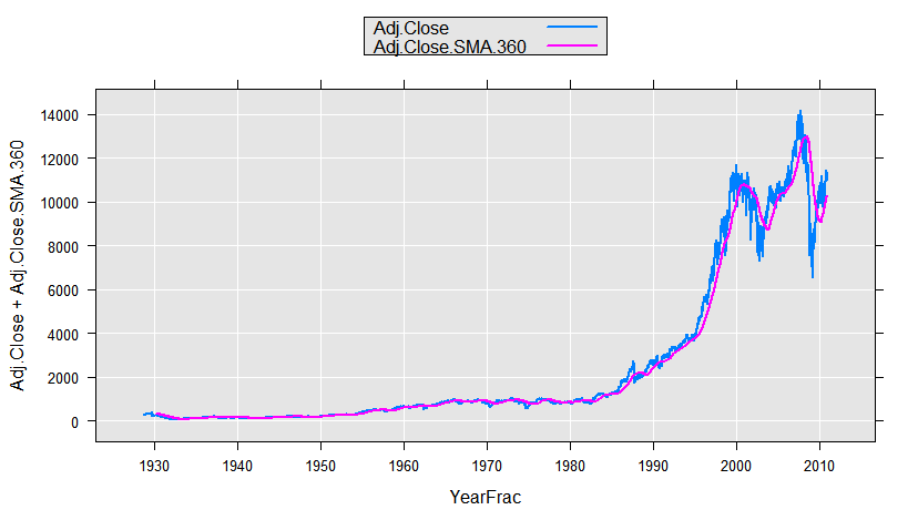
We could use this function with rxDataStep to add a variable to our data set, or on-the-fly, for example for plotting. Here we will use the sample data set containing daily information on the Dow Jones Industrial Average. We compute a 360-day moving average for the adjusted close (adjusted for dividends and stock splits) and plot it:
DJIAdaily <- file.path(rxGetOption("sampleDataDir"), "DJIAdaily.xdf")
rxLinePlot(Adj.Close+Adj.Close.SMA.360~YearFrac, data=DJIAdaily,
	transformFunc=makeMoveAveTransFunc(numDays=360),
	transformVars=c("Adj.Close"))
Extended example showing a series of transformations
A transforms argument can be a powerful way to effect a sequence of changes on a row by row basis. The transforms argument is specified as a list of expressions. Given R expressions operate row-by-row (that is, the computed value of the new variable for an observation is only dependent on values of other variables for that observation), you can combine them into a single transforms argument, as this example demonstrates.
Start with a simple data frame containing a small sample of transaction data:
#  Transforming Data with rxDataStep

expData <- data.frame(
	BuyDate = c("2011/10/1", "2011/10/1", "2011/10/1",
	"2011/10/2", "2011/10/2", "2011/10/2", "2011/10/2",
	"2011/10/3", "2011/10/4", "2011/10/4"),
	Food =      c( 32, 102,  34,  5,   0, 175,  15, 76, 23, 14),
	Wine =      c( 0,  212,   0,  0, 425,  22,   0, 12,  0, 56),
	Garden =    c( 0,   46,   0,  0,   0,  45, 223,  0,  0, 0),
	House = c( 22,  72,  56,  3,   0,  0,    0, 37, 48, 23),
	Sex =   factor(c("F", "F", "M", "M", "M", "F", "F", "F", "M", "F")),
	Age =          c( 20,  51,  32,  16,  61, 42,  35, 99, 29, 55),
	stringsAsFactors = FALSE)
Apply a series of data transformations:
- Compute the total expenditures for each store visit
- Compute the average category expenditure for each store visit
- Set the variable Age to missing if the value is 99
- Create a new logical variable UnderAge if the purchaser is under 21
- Find the day of week the purchase was made using R’s as.POSIXlt function, then convert it to a factor. [Note that when creating factors in a transform, you must specify the levels or you may get unpredictable results. Alternatively use rxFactors.]
- Create a factor variable for categories of expenditure levels
- Create a logical variable for expenditures of $50 or more on either Food or Wine
- Remove the variable BuyDate from the data set
The following call to rxDataStep will accomplish all of the above, returning a new data frame with the transformed variables:
newExpData = rxDataStep( inData = expData,
	transforms = list(
		Total      = Food + Wine + Garden + House,
		AveCat     = Total/4,
		Age        = ifelse(Age == 99, NA, Age),
		UnderAge   = Age < 21,
		Day        = (as.POSIXlt(BuyDate))$wday,
		Day        = factor(Day, levels = 0:6,
						labels = c("Su","M","Tu", "W", "Th","F", "Sa")),
		SpendCat   = cut(Total, breaks=c(0, 75, 250, 10000),
					labels=c("low", "medium", "high"), right=FALSE),
		FoodWine = ifelse( Food > 50, TRUE, FALSE),
		FoodWine = ifelse( Wine > 50, TRUE, FoodWine),
		BuyDate  = NULL))
newExpData
The new data frame shows all of the transformed data:
	   Food Wine Garden House Sex Age Total AveCat UnderAge Day SpendCat FoodWine
	1    32    0      0    22   F  20    54  13.50     TRUE  Sa      low    FALSE
	2   102  212     46    72   F  51   432 108.00    FALSE  Sa     high     TRUE
	3    34    0      0    56   M  32    90  22.50    FALSE  Sa   medium    FALSE
	4     5    0      0     3   M  16     8   2.00     TRUE  Su      low    FALSE
	5     0  425      0     0   M  61   425 106.25    FALSE  Su     high     TRUE
	6   175   22     45     0   F  42   242  60.50    FALSE  Su   medium     TRUE
	7    15    0    223     0   F  35   238  59.50    FALSE  Su   medium    FALSE
	8    76   12      0    37   F  NA   125  31.25       NA   M   medium     TRUE
	9    23    0      0    48   M  29    71  17.75    FALSE  Tu      low    FALSE
	10   14   56      0    23   F  55    93  23.25    FALSE  Tu   medium     TRUE
If we had a large data set containing expenditure data in an .xdf file, we could use exactly the same transformation code; the only changes in the call to rxDataStep would be the inData and the addition of an outFile for the newly created data set.
Next Steps
Continue on to the following data-related articles to learn more about XDF, data source objects, and other data formats:
- Data transformations (introduction)
- XDF files
- Data Sources
- Import text data
- Import ODBC data
- Import and consume data on HDFS
See Also
RevoScaleR Functions
Tutorial: data import and exploration
Tutorial: data visualization and analysis