Running jobs in parallel using rxExec

Important

This content is being retired and may not be updated in the future. The support for Machine Learning Server will end on July 1, 2022. For more information, see What's happening to Machine Learning Server?

RevoScaleR functions are engineered to execute in parallel automatically. However, if you require a custom implementation, you can use rxExec to manually construct and manage a distributed workload. With rxExec, you can take an arbitrary function and run it in parallel on your distributed computing resources in Hadoop. This in turn allows you to tackle a wide variety of parallel computing problems.

This article provides comprehensive steps on how to use rxExec, starting with examples showcasing rxExec in a variety of use cases.

Examples using rxExec

To demonstrate rxExec usage, this article provides several examples:

• Simulate a dice-rolling game
• Determine the probability that any two persons in a given group size share a birthday
• Create a plot of the Mandelbrot set
• Perform naive k-means clustering

In general, the only required arguments to rxExec are the function to be run and any required arguments of that function. Additional optional arguments can be used to control the computation.

Before trying the examples, be sure that your compute context is set with the option wait=TRUE.

Playing Dice: A Simulation

A familiar casino game consists of rolling a pair of dice. If you roll a 7 or 11 on your initial roll, you win. If you roll 2, 3, or 12, you lose. Roll a 4, 5, 6, 8, 9, or 10, NS that number becomes your point and you continue rolling until you either roll your point again (in which case you win) or roll a 7, in which case you lose. The game is easily simulated in R using the following function:

playDice <- function()
{
	result <- NULL
	point <- NULL
	count <- 1
	while (is.null(result))
	{
		roll <- sum(sample(6, 2, replace=TRUE))

		if (is.null(point))
		{
			point <- roll
		}
		if (count == 1 && (roll == 7 || roll == 11))
		{
			result <- "Win"
		}
		else if (count == 1 && (roll == 2 || roll == 3 || roll == 12))
		{
			result <- "Loss"
		}
		else if (count > 1 && roll == 7 )
		{
			result <- "Loss"
		}
		else if (count > 1 && point == roll)
		{
			result <- "Win"
		}
		else
		{
			count <- count + 1
		}
	}
	result
}

Using rxExec, you can invoke thousands of games to help determine the probability of a win. Using a Hadoop 5-node cluster, we play the game 10000 times, 2000 times on each node:

z <- rxExec(playDice, timesToRun=10000, taskChunkSize=2000)
table(unlist(z))

Loss  Win
5087 4913

We expect approximately 4929 wins in 10000 trials, and our result of 4913 wins is close.

The Birthday Problem

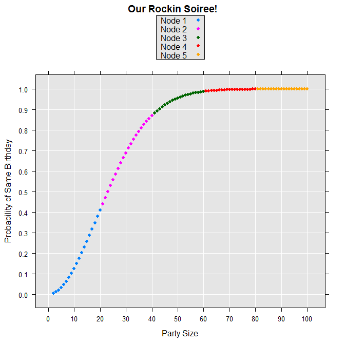
The birthday problem is an old standby in introductory statistics classes because its result seems counterintuitive. In a group of about 25 people, the chances are better than 50-50 that at least two people in the room share a birthday. Put 50 people in a room and you are practically guaranteed there is a birthday-sharing pair. Since 50 is so much less than 365, most people are surprised by this result.

We can use the following function to estimate the probability of at least one birthday-sharing pair in groups of various sizes (the first line of the function is what allows us to obtain results for more than one value at a time; the remaining calculations are for a single n):

"pbirthday" <- function(n, ntests=5000)
{   
	if (length(n) > 1L) return(sapply(n, pbirthday, ntests = ntests))

	daysInYear <- seq.int(365)
	anydup <- function(i)
	{
		any(duplicated(sample(daysInYear, size = n, replace = TRUE)))
	}

	prob <- sum(sapply(seq.int(ntests), anydup)) / ntests
	names(prob) <- n
	prob
}

We can test that it works in a sequential setting, estimating the probability for group sizes 3, 25, and 50 as follows:

pbirthday(c(3,25,50))

For each group size, 5000 random tests were performed. For this run, the following results were returned:

	     3     25     50
	0.0078 0.5710 0.9726

Make sure your compute context is set to a “waiting” context. Then distribute this computation for groups of 2 to 100 using rxExec as follows, using rxElemArg to specify a different argument for each call to pbirthday, and then using the taskChunkSize argument to pass these arguments to the nodes in chunks of 20:

z <- rxExec(pbirthday, n=rxElemArg(2:100), taskChunkSize=20)

The results are returned in a list, with one element for each node. We can use unlist to convert the results into a single vector:

probSameBD <- unlist(z)

We can make a colorful plot of the results by constructing variables for the party sizes and the nodes where each computation was performed:

partySize <- 2:100
nodes <- as.factor( rep(1:5, each=20)[2:100])
levels(nodes) <- paste("Node", levels(nodes))
birthdayData <- data.frame(probSameBD, partySize, nodes)

rxLinePlot( probSameBD~partySize, groups = nodes, data=birthdayData,
	type = "p",
	xTitle = "Party Size",
	yTitle = "Probability of Same Birthday",
	title = "Our Rockin Soiree!")

The resulting plot is shown as follows:

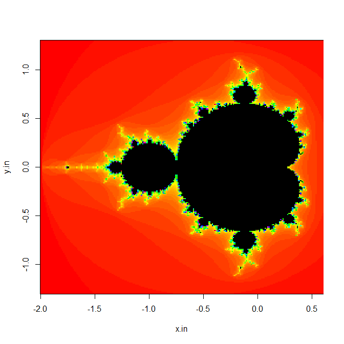
Plotting the Mandelbrot Set

Computing the Mandelbrot set is a popular parallel computing example because it involves a simple computation performed independently on an array of points in the complex plane. For any point z=x+yi in the complex plane, z belongs to the Mandelbrot set if and only if z remains bounded under the iteration z_(n+1)=z_n^2+z_n. If we are associating a point (x_0,y_0) in the plane with a pixel on a computer screen, the following R function returns the number of iterations before the point becomes unbounded, or the maximum number of iterations. If the maximum number of iterations is returned, the point is assumed to be in the set:

mandelbrot <- function(x0,y0,lim)
{
	x <- x0; y <- y0
	iter <- 0
	while (x^2 + y^2 < 4 && iter < lim)
	{
		xtemp <- x^2 - y^2 + x0
		y <- 2 * x * y + y0
		x <- xtemp
		iter <- iter + 1
	}
	iter
}

The following function retains the basic computation but returns a vector of results for a given y value:

vmandelbrot <- function(xvec, y0, lim)
{
	unlist(lapply(xvec, mandelbrot, y0=y0, lim=lim))
}

We can then distribute this computation by computing several rows at a time on each compute resource. In the following, we create an input x vector of length 240, a y vector of length 240, and specify the iteration limit as 100. We then call rxExec with our vmandelbrot function, giving 1/5 of the y vector to each computational node in our five node HPC Server cluster. This should be done in a compute context with wait=TRUE. Finally, we put the results into a 240x240 matrix and create an image plot that shows the familiar Mandelbrot set:

x.in <- seq(-2.0, 0.6, length.out=240)
y.in <- seq(-1.3, 1.3, length.out=240)
m <- 100
z <- rxExec(vmandelbrot, x.in,y0=rxElemArg(y.in), m, taskChunkSize=48,
		execObjects="mandelbrot")
z <- matrix(unlist(z), ncol=240)
image(x.in, y.in, z, col=c(rainbow(m), '#000000'), useRaster=TRUE)

The resulting plot is shown as follows (not all graphics devices support the useRaster argument; if your plot is empty, try omitting that argument):

### Naïve Parallel k-Means Clustering

RevoScaleR has a built-in analysis function, rxKmeans, to perform distributed k-means, but in this section we see how the regular R kmeans function can be put to use in a distributed context.

The kmeans function implements several iterative relocation algorithms for clustering. An iterative relocation algorithm starts from an initial classification and then iteratively moves data points from one cluster to another to reduce sums of squares. One possible starting point is to pick cluster centers at random and then assign points to each cluster so that the sum of squares is minimized. If this procedure is repeated many times for different sets of centers, the set with the smallest error can be chosen.

We can do this with the ordinary kmeans function, which has a parameter nstart that tells it how many times to pick the starting centers, and also to pick the set of centers that returns a result with smallest error:     x <- matrix(rnorm(250000), nrow = 5000, ncol = 50)     system.time(kmeans(x, centers=10, iter.max = 35, nstart = 400))

On a Dell XPS laptop with 8 GB of RAM, this takes about a minute and a half.

To parallelize this computation efficiently, we should do the following:

- Pass the data to a specified number of computing resources once.

- Split the work into smaller tasks for passing to each computing resource.

- Combine the results from all the computing resources so the best result is returned.

In the case of kmeans, we can ask for the computations to be done by cores, rather than by nodes. Because we are distributing the computation, we can do fewer repetitions (nstarts) on each compute element. We can do all of this with the following function (again, this should be run with a compute context for which wait=TRUE):

    kMeansRSR <- function(x, centers=5, iter.max=10, nstart=1)
    {
        numTimes <- 20
        results <- rxExec(FUN = kmeans, x=x, centers=centers, iter.max=iter.max,
            nstart=nstart, timesToRun=numTimes)
        best <- 1
        bestSS <- sum(results[[1]]$withinss)
        for (j in 1:numTimes)
        {
              jSS <- sum(results[[j]]$withinss)
              if (bestSS > jSS)
              {
                      best <- j
                     bestSS <- jSS
              }
        }
        results[[best]]
    }

Notice that in our kMeansRSR function we are letting the underlying kmeans function find nstart sets of centers per call and the choice of "best" is done in our function after we have called kmeans numTimes. No parallelization is done to kmeans itself.

With our kMeansRSR function, we can then repeat the computation from before:

system.time(kMeansRSR(x, 10, 35, 20))

With our 5-node HPC Server cluster, this reduces the time from a minute and a half to about 15 seconds.

Share data across parallel processes

Data can be shared between rxExec parallel processes by copying it to the environment of each process through the execObjects option to rxExec, or by specifying the data as arguments to each function call. For small data, this works well but as the data objects get larger this can create a significant performance penalty due to the time needed to do the copy. In such cases, it can be much more efficient to share the data by storing it in a location accessible by each of the parallel processes, such as a local or network file share.

The following example shows how this can be done when parallelizing the computation of statistics on subsets of a larger data table.

We’ll start by creating some sample data using the data.table package.

	library(data.table)

	nrows <- 5e6
	test.data  <- data.table(tag=sample(LETTERS[1:7], nrows, replace=TRUE), 
							a=runif(nrows), b=runif(nrows))

	# get the unique tags that we'll subset by 
	tags <- unique(test.data$tag)
	tags

Next we’ll setup for use of the doParallel backend.

	library(doParallel) 
	(nCore <- parallel::detectCores(all.tests = TRUE, logical = FALSE) )
	cl <- makeCluster(nCore, useXDR = F)
	registerDoParallel(cl)
	rxSetComputeContext(RxForeachDoPar())

	# set MKL thread to 1 to avoid contention 
	setMKLthreads(1)  

Now we create a function for computing statistics on a selected subset of the data table by passing in both the data table and the tag value to subset by. We’ll then run the function using rxExec for each tag value.

	filterTest <- function(d, ztag) {
	sum(subset(d, tag==ztag, select=a)) 
	}
	system.time({
	res1 <- rxExec(filterTest, test.data, rxElemArg(tags))
	}) 
	##   user  system elapsed 
	##   9.67    7.40   22.05 

To see the impact of sharing the file via a common storage location rather than passing it to each parallel process we’ll save the data table into an RDS file, which is an efficient way of storing individual R objects, create a new version of the function that reads the data table from the RDS file, and then rerun rxExec using the new function.

	saveRDS(test.data, 'c:/temp/tmp.rds', compress=FALSE)
	filterTest <- function(ztag) {
	d <- readRDS('c:/temp/tmp.rds')
	sum(subset(d, tag==ztag, select=a)) 
	}

	system.time({
	res2 <- rxExec(filterTest, rxElemArg(tags))
	}) 
	##   user  system elapsed 
	##   0.03    0.00   11.01 

	# make sure the results match 
	identical(res2, res2)  
	## [1] TRUE 

	# close up shop 
	stopCluster(cl)

Although results may vary, in this case we’ve reduced the elapsed time by 50% by sharing the data table rather than passing it as an in-memory object to each parallel process.

Parallel Random Number Generation

When generating random numbers in parallel computation, a frequent problem is the possibility of highly correlated random number streams. High-quality parallel random number generators avoid this problem. RevoScaleR includes several high-quality parallel random number generators and these can be used with rxExec to improve the quality of your parallel simulations.

By default, a parallel version of the Mersenne-Twister random number generator is used that supports 6024 separate substreams. We can set it to work on our dice example by setting a non-null seed:

z <- rxExec(playDice, timesToRun=10000, taskChunkSize=2000, RNGseed=777)
table(unlist(z))

This makes our simulation repeatable:

Loss  Win
5104 4896

z <- rxExec(playDice, timesToRun=10000, taskChunkSize=2000, RNGseed=777)
table(unlist(z))

Loss  Win
5104 4896

This random number generator can be asked for explicitly by specifying RNGkind="MT2203":

z <- rxExec(playDice, timesToRun=10000, taskChunkSize=2000, RNGseed=777,
	RNGkind="MT2203")
table(unlist(z))

Loss  Win
5104 4896

We can build reproducibility into our naïve k-means example as follows:

kMeansRSR <- function(x, centers=5, iter.max=10, nstart=1, numTimes = 20, seed = NULL)
{
	results <- rxExec(FUN = kmeans, x=x, centers=centers, iter.max=iter.max,
		nstart=nstart, timesToRun=numTimes, RNGseed = seed)
	best <- 1
	bestSS <- sum(results[[1]]$withinss)
	for (j in 1:numTimes)
	{
			jSS <- sum(results[[j]]$withinss)
			if (bestSS > jSS)
			{
					best <- j
					bestSS <- jSS
			}
	}
	results[[best]]
}
km1 <- kMeansRSR(x, 10, 35, 20, seed=777)
km2 <- kMeansRSR(x, 10, 35, 20, seed=777)
all.equal(km1, km2)

	[1] TRUE

To obtain the default random number generators without setting a seed, specify "auto" as the argument to either RNGseed or RNGkind:

x3 <- rxExec(runif, 500, timesToRun=5, RNGkind="auto")
x4 <- rxExec(runif, 500, timesToRun=5, RNGseed="auto")

To verify that we are actually getting uncorrelated streams, we can use runif within rxExec to generate a list of vectors of random vectors, then use the cor function to measure the correlation between vectors:

x <- rxExec(runif, 500, timesToRun=5, RNGkind="MT2203")
x.df <- data.frame(x)
corx <- cor(x.df)
diag(corx) <- 0
any(abs(corx)> 0.3)

Correlations are above 0.3; in repeated runs of the code, the maximum correlation seldom exceeded 0.1.

Because the MT2203 generator offers such a rich array of substreams, we recommend its use. You can, however, use several other generators, all from Intel’s Vector Statistical Library, a component of the Intel Math Kernel Library. The available generators are as follows: "MCG31", "R250", "MRG32K3A", "MCG59", "MT19937", "MT2203", "SFMT19937" (all of which are pseudo-random number generators that can be used to generate uncorrelated random number streams) plus "SOBOL" and "NIEDERR", which are quasi-random number generators that do not generate uncorrelated random number streams. Detailed descriptions of the available generators can be found in the Vector Statistical Library Notes.

About reproducibility

For distributed compute contexts, rxExec starts the random number streams on a per-worker basis; if there are more tasks than workers, you may not obtain completely reproducible results because different tasks may be performed by randomly chosen workers. If you need completely reproducible results, you can use the taskChunkSize argument to force the number of task chunks to be less than or equal to the number of workers. This will ensure that each chunk of tasks is performed on a single random number stream. You can also define a custom function that includes random number generation control within it; this moves the random number control into each task. See the help file for rxRngNewStream for details.

Work with results from non-blocking jobs

So far, all of our examples have required a blocking, or waiting, compute context so that we could make immediate use of the results returned by rxExec. However some computations are so time consuming that it is not practical to wait on the results. In such cases, it is probably best to divide your analysis into two or more pieces, one of which can be structured as a non-blocking job, and then use the pending job (or more usefully, the job results, when available) as input to the remaining pieces.

For example, let’s return to the birthday example, and see how to restructure our analysis to use a non-blocking job for the distributed computations. The pbirthday function itself requires no changes, and our variable specifying the number of ntests can be used as is:

"pbirthday" <- function(n, ntests=5000)
{   
	if (length(n) > 1L) return(sapply(n, pbirthday, ntests = ntests))

	daysInYear <- seq.int(365)
	anydup <- function(i)
	{
		any(duplicated(sample(daysInYear, size = n, replace = TRUE)))
	}

	prob <- sum(sapply(seq.int(ntests), anydup)) / ntests
	names(prob) <- n
	prob
}
ntests <- 2000

However, when we call rxExec, the return object will no longer be the results list, but a jobInfo object:

z <- rxExec(pbirthday, n=rxElemArg(2:100), ntests=ntests, taskChunkSize=20)

We check the job status:

rxGetJobStatus(z)

	[1] "finished"

We can then proceed almost as before:

probSameBD <- unlist(rxGetJobResults(z))
partySize <- 2:100
nodes = as.factor( rep(1:5, each=20)[2:100])
levels(nodes) <- paste("Node", levels(nodes))
birthdayData <- data.frame(probSameBD, partySize, nodes)

rxLinePlot( probSameBD~partySize, groups = nodes, data=birthdayData,
	type = "p",
	xTitle = "Party Size",
	yTitle = "Probability of Same Birthday",
	title = "Our Rockin Soiree!")

The other examples are a bit trickier, in that the result of the calls to rxExec were embedded in functions. But again, dividing the computations into distributed and non-distributed components can help—the distributed computations can be non-blocking, and the non-distributed portions can then be applied to the results. Thus the kmeans example can be rewritten thus:

genKmeansClusters <- function(x, centers=5, iter.max=10, nstart=1)
{
	numTimes <- 20
	rxExec(FUN = kmeans, x=x, centers=centers, iter.max=iter.max,
		nstart=nstart, timesToRun=numTimes)
}

findKmeansBest <- function(results){
	numTimes <- length(results)
	best <- 1
	bestSS <- sum(results[[1]]$withinss)
	for (j in 1:numTimes)
	{
			jSS <- sum(results[[j]]$withinss)
			if (bestSS > jSS)
			{
					best <- j
					bestSS <- jSS
			}
	}
	results[[best]]
}

To run this in our non-blocking cluster context, we do the following:

x <- matrix(rnorm(250000), nrow = 5000, ncol = 50)
z <- genKmeansClusters(x, 10, 35, 20)

Once we see that z’s job status is “finished”, we can run findKmeansBest on the results:

findKmeansBest(rxGetJobResults(z))

Call RevoScaleR HPA functions with rxExec

To this point, none of the functions we have called with rxExec has been a RevoScaleR function, because the intent has been to show how rxExec can be used to address the large class of traditional high-performance computing problems.

However, there is no inherent reason why rxExec cannot be used with RevoScaleR’s high performance analysis (HPA) functions, and many times it can be useful to do so. For example, if you are running a cluster on which every node has two or more cores, you can use rxExec to start an independent analysis on each node, and each of those analyses can take advantage of the multiple cores on its node.

The following simulation simulates data from a Poisson distribution and then fits a generalized linear model to the simulated data:

"SimAndEstimatePoisson" <- function(nobs, trials)
{
	"SimulatePoissonData" <- function(nobs)
	{
		x1 <- log(runif(nobs, min=.5, max=1.5))
		x2 <- log(runif(nobs, min=.5, max=1.5))

		b0 <- 0
		b1 <- 1
		b2 <- 2
		lambda <- exp(b0 + b1*x1 + b2*x2)
		count <- rpois(nobs,lambda)
		pSim <- data.frame(count=count, x1=x1, x2=x2)
	}

	cf <- NULL
	rxOptions(reportProgress = 0)
	for (i in 1:trials)
	{
		simData <- SimulatePoissonData(nobs)
		result1 <- rxGlm(count~x1+x2,data=simData,family=poisson())
		cf <- rbind(cf,as.double(coefficients(result1)))
	}
	cf       
}

If we call the above function with rxExec on a five-node cluster compute context, we get five simulations running simultaneously, and can easily produce 1000 simulations as follows:

rxExec(SimAndEstimatePoisson, nobs=50000, trials=10, taskChunkSize=5, timesToRun=100)

It is important to recognize the distinction between running an HPA function with a distributed compute context, and calling an HPA function using rxExec with a distributed compute context. In the former case, we are fitting just one model, using the distributed compute context to farm out portions of the computations, but ultimately returning just one model object. In the latter case, we are calculating one model per task, the tasks being farmed out to the various nodes or cores as desired, and a list of models is returned.

Use rxExec in the local compute context

By default, if you call rxExec in the local compute context, your computation runS sequentially on your local machine. However, you can incorporate parallel computing on your local machine using the special compute context RxLocalParallel as follows:

rxSetComputeContext(RxLocalParallel())

This allows the ParallelR package doParallel to distribute the computation among the available cores of your computer.

If you are using random numbers in the local parallel context, be aware that rxExec chooses a number of workers based on the number of tasks and the current value of rxGetOption("numCoresToUse"). to guarantee each task runS with a separate random number stream, set rxOptions(numCoresToUse) equal to the number of tasks, and explicitly set timesToRun to the number of tasks. For example, if we want a list consisting of five sets of uniform random numbers, we could do the following to obtain reproducible results:

rxOptions(numCoresToUse=5)
x1 <- rxExec(runif, 500, timesToRun=5, RNGkind="MT2203", RNGseed=14)
x2 <- rxExec(runif, 500, timesToRun=5, RNGkind="MT2203", RNGseed=14)
all.equal(x1, x2)

numCoresToUse is a scalar integer specifying the number of cores to use. If you set this parameter to either -1 or a value in excess of available cores, ScaleR uses however many cores are available. Increasing the number of cores also increases the amount of memory required for ScaleR analysis functions.

Note

HPA functions are not affected by the RxLocalParallel compute context; they run locally and in the usual internally distributed fashion when the RxLocalParallel compute context is in effect.

Use rxExec with foreach back ends

If you do not have access to a Hadoop cluster or enterprise database, but do have access to a cluster via PVM, MPI, socket, or NetWorkSpaces connections or a multicore workstation, you can use rxExec with an arbitrary foreach backend (doParallel, doSNOW, doMPI, etc.) Register your parallel backend as usual and then set your RevoScaleR compute context using the special compute context RxForeachDoPar:

rxSetComputeContext(RxForeachDoPar())

For example, here is how you might start a SNOW-like cluster connection with the doParallel back end:

library(doParallel)
cl <- makeCluster(4)
registerDoParallel(cl)
rxSetComputeContext(RxForeachDoPar())

You then call rxExec as usual. The computations are automatically directed to the registered foreach back end.

Warning

HPA functions are not usually affected by the RxForeachDoPar compute context; they run locally and in the usual internally distributed fashion when the RxForeachDoPar compute context is in effect. The one exception is when HPA functions are called within rxExec; in this case it is possible that the internal threading of the HPA functions can be affected by the launch mechanism of the parallel backend workers. The doMC backend and the multicore-like backend of doParallel both use forking to launch their workers; this is known to be incompatible with the HPA functions.

Control rxExec computations

As we have seen in these examples, there are several arguments to rxExec that allow you to fine-tune your rxExec commands. Both the birthday example and the Mandelbrot example used the taskChunkSize argument to specify how many tasks should go to each worker. The Mandelbrot example also used the execObjects argument, which can be used to pass either a character vector or an environment containing objects—the objects specified by the vector or contained in the environment are added to the environment of the function specified in the FUN argument, unless that environment is locked, in which case they are added to the parent frame in which FUN is evaluated. (If you use an environment, it should be one you create with parent=emptyenv(); this allows you to pass only those objects you need to the function’s environment.) These two examples also show the use of rxElemArg in passing arguments to the workers. In the kmeans example, we covered the timesToRun argument. The packagesToLoad argument allows you to specify packages to load on each worker. The consoleOutput and autoCleanup flags serve the same purpose as their counterparts in the compute context constructor functions—that is, they can be used to specify whether console output should be displayed or the associated task files should be cleaned up on job completion for an individual call to 'rxExec'.

Two additional arguments remain to be introduced: oncePerElem and continueOnFailure. The oncePerElem argument restricts the called function to be run once per allotted node; this is frequently used with the timesToRun argument to ensure that each occurrence is run on a separate node. The oncePerElem argument, however, can only be set to TRUE if elemType="nodes". It must be set to FALSE if elemType="cores".

If oncePerElem is TRUE and elemType="nodes", rxExec’s results are returned in a list with components named by node. If a given node does not have a valid R syntactic name, its name is mangled to become a valid R syntactic name for use in the return list.

The continueOnFailure argument is used to say that a computation should continue even if one or more of the compute elements fails for some reason; this is useful, for example, if you are running several thousand independent simulations and It doesn’t matter if you get results for all of them. Using continueOnFailure=TRUE (the default), you get results for all compute elements that finish the simulation and error messages for the compute elements that fail.

Note

The arguments elemType, consoleOutput, autoCleanup, continueOnFailure, and oncePerElem are ignored by the special compute contexts 'RxLocalParallel' and 'RxForeachDoPar`.

Conclusion

This article provides comprehensive documentation on rxExec for writing custom script that executes jobs in parallel. Several use cases were used to show how rxExec is used in context, with additional sections providing guidance on relevant tasks associated with custom execution, such as sharing data, structuring jobs, and controlling calculations. To learn more, see these related links:

• Distributed and parallel computing in Machine Learning Server
• Using foreach and iterators for manual parallel execution
• Parallel execution using doRSR for script containing RevoScaleR and foreach constructs