Note
Access to this page requires authorization. You can try signing in or changing directories.
Access to this page requires authorization. You can try changing directories.
Conditional formatting in Excel applies formatting to cells based on specific conditions or rules. These formats automatically adjust when the data changes, so your script doesn't need to be run multiple times. This page contains a collection of Office Scripts that demonstrate various conditional formatting options.
This sample workbook contains worksheets ready to test with the sample scripts.
Note
Run these samples directly from the Office Scripts Code Editor. To open the Code Editor, go to Automate > New Script > Create in Code Editor. Replace the default code with the sample code you want to run, and then select Run.
Cell value
Cell value conditional formatting applies a format to every cell that contains a value meeting a given criteria. This helps quickly spot important data points.
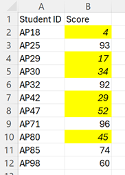
The following sample applies cell value conditional formatting to a range. Any value less than 60 will have the cell's fill color changed and the font made italic.
function main(workbook: ExcelScript.Workbook) {
    // Get the range to format.
    const sheet = workbook.getWorksheet("CellValue");
    const ratingColumn = sheet.getRange("B2:B12");
    sheet.activate();

    // Add cell value conditional formatting.
    const cellValueConditionalFormatting =
        ratingColumn.addConditionalFormat(ExcelScript.ConditionalFormatType.cellValue).getCellValue();

    // Create the condition, in this case when the cell value is less than 60
    let rule: ExcelScript.ConditionalCellValueRule = {
        formula1: "60",
        operator: ExcelScript.ConditionalCellValueOperator.lessThan
    };
    cellValueConditionalFormatting.setRule(rule);

    // Set the format to apply when the condition is met.
    let format = cellValueConditionalFormatting.getFormat();
    format.getFill().setColor("yellow");
    format.getFont().setItalic(true);
}
Color scale
Color scale conditional formatting applies a color gradient across a range. The cells with the minimum and maximum values of the range use the colors specified, with other cells scaled proportionally. An optional midpoint color provides more contrast.
This following sample applies a red, white, and blue color scale to the selected range.

function main(workbook: ExcelScript.Workbook) {
    // Get the range to format.
    const sheet = workbook.getWorksheet("ColorScale");
    const dataRange = sheet.getRange("B2:M13");
    sheet.activate();

    // Create a new conditional formatting object by adding one to the range.
    const conditionalFormatting = dataRange.addConditionalFormat(ExcelScript.ConditionalFormatType.colorScale);

    // Set the colors for the three parts of the scale: minimum, midpoint, and maximum.
    conditionalFormatting.getColorScale().setCriteria({
        minimum: {
            color: "#5A8AC6", /* A pale blue. */
            type: ExcelScript.ConditionalFormatColorCriterionType.lowestValue
        },
        midpoint: {
            color: "#FCFCFF", /* Slightly off-white. */
            formula: '=50', type: ExcelScript.ConditionalFormatColorCriterionType.percentile
        },
        maximum: {
            color: "#F8696B", /* A pale red. */
            type: ExcelScript.ConditionalFormatColorCriterionType.highestValue
        }
    });
}
Data bar
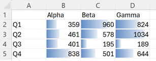
Data bar conditional formatting adds a partially-filled bar in the background of a cell. The fullness of the bar is defined by the value in the cell and the range specified by the format.
The following sample creates data bar conditional formatting on the selected ranged. The scale of the data bar goes from 0 to 1200.
function main(workbook: ExcelScript.Workbook) {
    // Get the range to format.
    const sheet = workbook.getWorksheet("DataBar");
    const dataRange = sheet.getRange("B2:D5");
    sheet.activate();

    // Create new conditional formatting on the range.
    const format = dataRange.addConditionalFormat(ExcelScript.ConditionalFormatType.dataBar);
    const dataBarFormat = format.getDataBar();

    // Set the lower bound of the data bar formatting to be 0.
    const lowerBound: ExcelScript.ConditionalDataBarRule = {
        type: ExcelScript.ConditionalFormatRuleType.number,
        formula: "0"
    };
    dataBarFormat.setLowerBoundRule(lowerBound);

    // Set the upper bound of the data bar formatting to be 1200.
    const upperBound: ExcelScript.ConditionalDataBarRule = {
        type: ExcelScript.ConditionalFormatRuleType.number,
        formula: "1200"
    };
    dataBarFormat.setUpperBoundRule(upperBound);
}
Icon set
Icon set conditional formatting adds icons to each cell in a range. The icons come from a specified set. Icons are applied based on an ordered array of criteria, with each criterion mapping to a single icon.
The following sample applies the "three traffic light" icon set conditional formatting to a range.
![]()
function main(workbook: ExcelScript.Workbook) {
    // Get the range to format.
    const sheet = workbook.getWorksheet("IconSet");
    const dataRange = sheet.getRange("B2:B12");
    sheet.activate();

    // Create icon set conditional formatting on the range.
    const conditionalFormatting = dataRange.addConditionalFormat(ExcelScript.ConditionalFormatType.iconSet);

    // Use the "3 Traffic Lights (Unrimmed)" set.
    conditionalFormatting.getIconSet().setStyle(ExcelScript.IconSet.threeTrafficLights1);
    conditionalFormatting.getIconSet().setCriteria([
      { // Use the red light as the default for positive values.
        formula: '=0', operator: ExcelScript.ConditionalIconCriterionOperator.greaterThanOrEqual,
        type: ExcelScript.ConditionalFormatIconRuleType.number
      },
      { // The yellow light is applied to all values 6 and greater. The replaces the red light when applicable.
        formula: '=6', operator: ExcelScript.ConditionalIconCriterionOperator.greaterThanOrEqual,
        type: ExcelScript.ConditionalFormatIconRuleType.number
      },
      { // The green light is applied to all values 8 and greater. As with the yellow light, the icon is replaced when the new criteria is met.
        formula: '=8', operator: ExcelScript.ConditionalIconCriterionOperator.greaterThanOrEqual,
        type: ExcelScript.ConditionalFormatIconRuleType.number
      }
    ]);
}
Preset
Preset conditional formatting applies a specified format to a range based on common scenarios, such as blank cells and duplicate values. The full list of preset criteria is provided by the ConditionalFormatPresetCriterion enum.
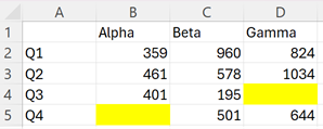
The following sample gives a yellow fill to any blank cell in the range.
function main(workbook: ExcelScript.Workbook) {
    // Get the range to format.
    const sheet = workbook.getWorksheet("Preset");
    const dataRange = sheet.getRange("B2:D5");
    sheet.activate();

    // Add new conditional formatting to that range.
    const conditionalFormat = dataRange.addConditionalFormat(
    ExcelScript.ConditionalFormatType.presetCriteria);

    // Set the conditional formatting to apply a yellow fill.
    const presetFormat = conditionalFormat.getPreset();
    presetFormat.getFormat().getFill().setColor("yellow");

    // Set a rule to apply the conditional format when cells are left blank.
    const blankRule: ExcelScript.ConditionalPresetCriteriaRule = {
        criterion: ExcelScript.ConditionalFormatPresetCriterion.blanks
    };
    presetFormat.setRule(blankRule);
}
Text comparison
Text comparison conditional formatting formats cells based on their text content. The formatting is applied when the text begins with, contains, ends with, or doesn't contain the given substring.
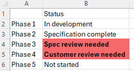
The following sample marks any cell in the range that contains the text "review".
function main(workbook: ExcelScript.Workbook) {
    // Get the range to format.
    const sheet = workbook.getWorksheet("TextComparison");
    const dataRange = sheet.getRange("B2:B6");
    sheet.activate();

    // Add conditional formatting based on the text in the cells.
    const textConditionFormat = dataRange.addConditionalFormat(
        ExcelScript.ConditionalFormatType.containsText).getTextComparison();

    // Set the conditional format to provide a light red fill and make the font bold.
    textConditionFormat.getFormat().getFill().setColor("#F8696B");
    textConditionFormat.getFormat().getFont().setBold(true);

    // Apply the condition rule that the text contains with "review".
    const textRule: ExcelScript.ConditionalTextComparisonRule = {
        operator: ExcelScript.ConditionalTextOperator.contains,
        text: "review"
    };
    textConditionFormat.setRule(textRule);
}
Top/bottom
Top/bottom conditional formatting marks the highest or lowest values in a range. The highs and lows are based on either raw values or percentages.
The following sample applies conditional formatting to show the two highest numbers in the range.
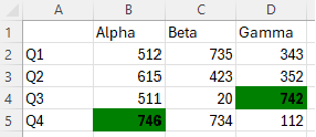
function main(workbook: ExcelScript.Workbook) {
  // Get the range to format.
  const sheet = workbook.getWorksheet("TopBottom");
  const dataRange = sheet.getRange("B2:D5");
  sheet.activate();

    // Set the fill color to green and the font to bold for the top 2 values in the range.
    const topBottomFormat = dataRange.addConditionalFormat(ExcelScript.ConditionalFormatType.topBottom).getTopBottom();
    topBottomFormat.getFormat().getFill().setColor("green");
    topBottomFormat.getFormat().getFont().setBold(true);
    topBottomFormat.setRule({
      rank: 2, /* The numeric threshold. */
      type: ExcelScript.ConditionalTopBottomCriterionType.topItems /* The type of the top/bottom condition. */
    });
}
Custom conditions
Custom conditional formatting allows for complex formulas to define when formatting is applied. Use this when the other options aren't enough.
The following sample sets a custom conditional formatting on the selected range. A light-green fill and bold font are applied to a cell if the value is larger than the value in the row's previous column.

function main(workbook: ExcelScript.Workbook) {
    // Get the range to format.
    const sheet = workbook.getWorksheet("Custom");
    const dataRange = sheet.getRange("B2:H2");
    sheet.activate();

    // Apply a rule for positive change from the previous column.
    const positiveChange = dataRange.addConditionalFormat(ExcelScript.ConditionalFormatType.custom).getCustom();
    positiveChange.getFormat().getFill().setColor("lightgreen");
    positiveChange.getFormat().getFont().setBold(true);
    positiveChange.getRule().setFormula(
        `=${dataRange.getCell(0, 0).getAddress()}>${dataRange.getOffsetRange(0, -1).getCell(0, 0).getAddress()}`
    );
}
Office Scripts