Computed table scenarios and use cases
There are benefits to using computed tables in a dataflow. This article describes use cases for computed tables and describes how they work behind the scenes.
What is a computed table?
A table represents the data output of a query created in a dataflow, after the dataflow has been refreshed. It represents data from a source and, optionally, the transformations that were applied to it. Sometimes, you might want to create new tables that are a function of a previously ingested table.
Although it's possible to repeat the queries that created a table and apply new transformations to them, this approach has drawbacks: data is ingested twice, and the load on the data source is doubled.
Computed tables solve both problems. Computed tables are similar to other tables in that they get data from a source and you can apply further transformations to create them. But their data originates from the storage dataflow used, and not the original data source. That is, they were previously created by a dataflow and then reused.
Computed tables can be created by referencing a table in the same dataflow or by referencing a table created in a different dataflow.

Why use a computed table?
Performing all transformation steps in one table can be slow. There can be many reasons for this slowdown—the data source might be slow, or the transformations that you're doing might need to be replicated in two or more queries. It might be advantageous to first ingest the data from the source and then reuse it in one or more tables. In such cases, you might choose to create two tables: one that gets data from the data source, and another—a computed table—that applies more transformations to data already written into the data lake used by a dataflow. This change can increase performance and reusability of data, saving time and resources.
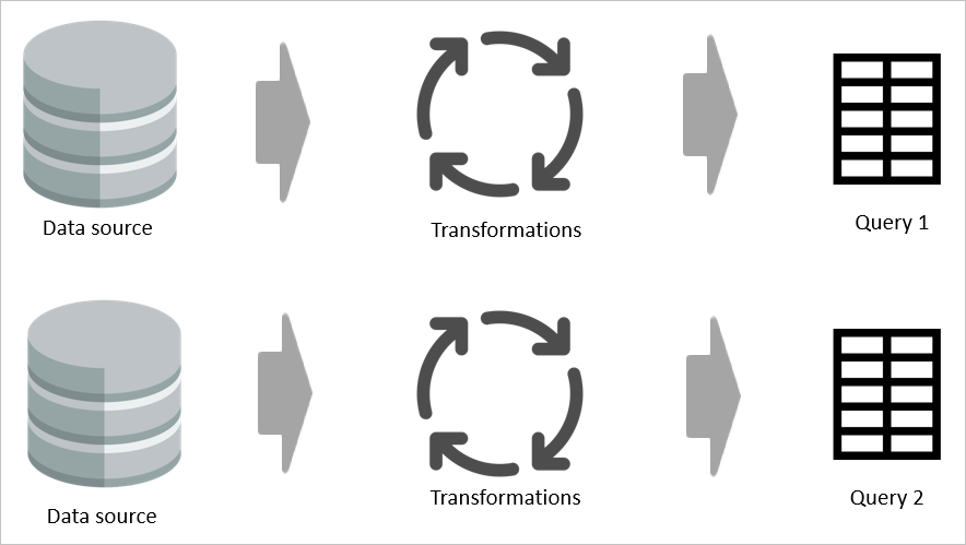
For example, if two tables share even a part of their transformation logic, without a computed table, the transformation has to be done twice.
However, if a computed table is used, then the common (shared) part of the transformation is processed once and stored in Azure Data Lake Storage. The remaining transformations are then be processed from the output of the common transformation. Overall, this processing is much faster.
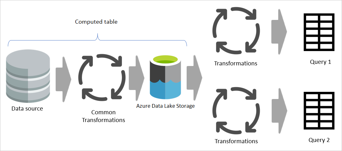
A computed table provides one place as the source code for the transformation and speeds up the transformation because it only needs to be done once instead of multiple times. The load on the data source is also reduced.
Example scenario for using a computed table
If you're building an aggregated table in Power BI to speed up the data model, you can build the aggregated table by referencing the original table and applying more transformations to it. By using this approach, you don't need to replicate your transformation from the source (the part that is from the original table).
For example, the following figure shows an Orders table.

Using a reference from this table, you can build a computed table.
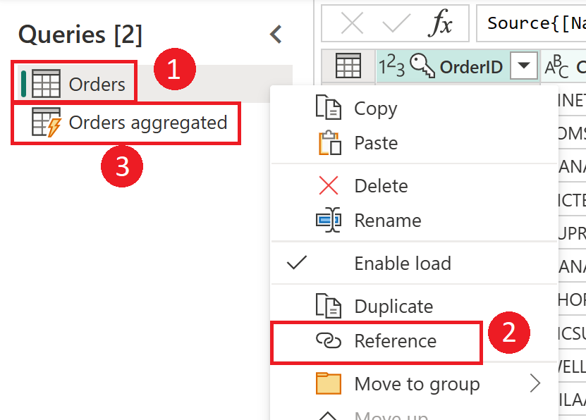
Screenshot showing how to create a computed table from the Orders table. First right-click the Orders table in the Queries pane, select the Reference option from the drop-down menu. This action creates the computed table, which is renamed here to Orders aggregated.
The computed table can have further transformations. For example, you can use Group By to aggregate the data at the customer level.
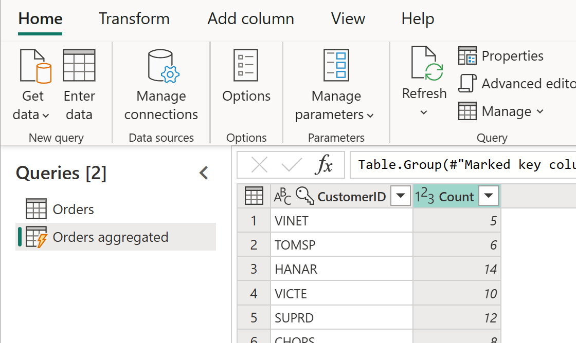
This means that the Orders Aggregated table is getting data from the Orders table, and not from the data source again. Because some of the transformations that need to be done have already been done in the Orders table, performance is better and data transformation is faster.
Computed table in other dataflows
You can also create a computed table in other dataflows. It can be created by getting data from a dataflow with the Microsoft Power Platform dataflow connector.
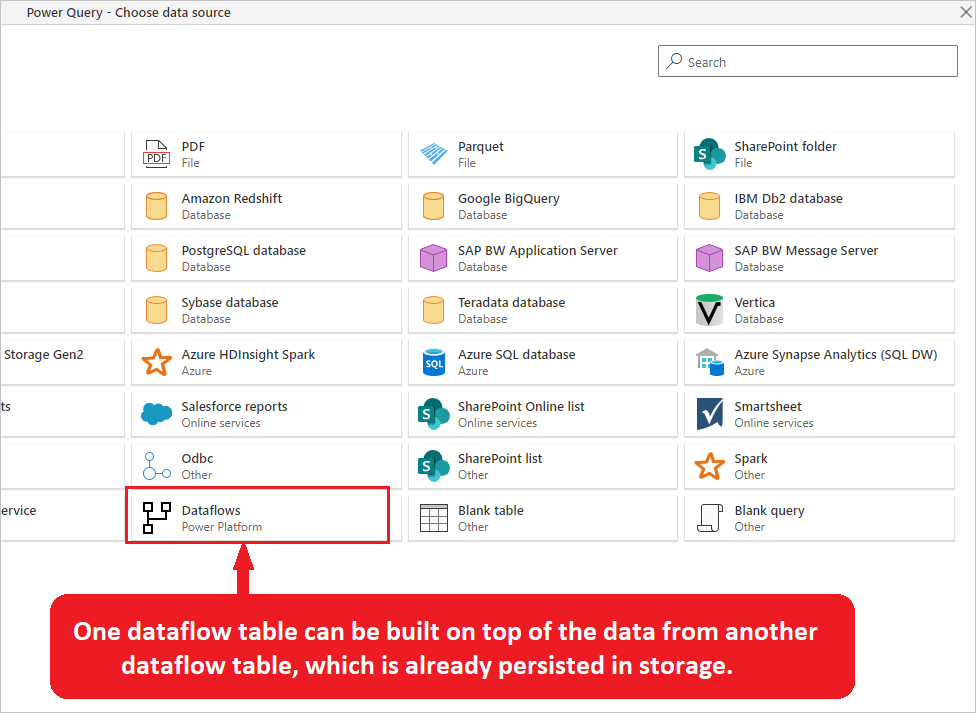
Image emphasizes the Power Platform dataflows connector from the Power Query choose data source window. Also included is a description that states that one dataflow table can be built on top of the data from another dataflow table, which is already persisted in storage.
The concept of the computed table is to have a table persisted in storage, and other tables sourced from it, so that you can reduce the read time from the data source and share some of the common transformations. This reduction can be achieved by getting data from other dataflows through the dataflow connector or referencing another query in the same dataflow.
Computed table: With transformations, or without?
Now that you know computed tables are great for improving performance of the data transformation, a good question to ask is whether transformations should always be deferred to the computed table or whether they should be applied to the source table. That is, should data always be ingested into one table and then transformed in a computed table? What are the pros and cons?
Load data without transformation for Text/CSV files
When a data source doesn't support query folding (such as Text/CSV files), there's little benefit in applying transformations when getting data from the source, especially if data volumes are large. The source table should just load data from the Text/CSV file without applying any transformations. Then, computed tables can get data from the source table and perform the transformation on top of the ingested data.
You might ask, what's the value of creating a source table that only ingests data? Such a table can still be useful, because if the data from the source is used in more than one table, it reduces the load on the data source. In addition, data can now be reused by other people and dataflows. Computed tables are especially useful in scenarios where the data volume is large, or when a data source is accessed through an on-premises data gateway, because they reduce the traffic from the gateway and the load on data sources behind them.
Doing some of the common transformations for a SQL table
If your data source supports query folding, it's good to perform some of the transformations in the source table because the query is folded to the data source, and only the transformed data is fetched from it. These changes improve overall performance. The set of transformations that is common in downstream computed tables should be applied in the source table, so they can be folded to the source. Other transformations that only apply to downstream tables should be done in computed tables.
Feedback
Coming soon: Throughout 2024 we will be phasing out GitHub Issues as the feedback mechanism for content and replacing it with a new feedback system. For more information see: https://aka.ms/ContentUserFeedback.
Submit and view feedback for