Note
Access to this page requires authorization. You can try signing in or changing directories.
Access to this page requires authorization. You can try changing directories.
Applies to: ![]() SQL Server 2016 (13.x) and later versions
SQL Server 2016 (13.x) and later versions ![]() Azure SQL Managed Instance
Azure SQL Managed Instance
In part three of this four-part tutorial series, you'll build a K-Means model in R to perform clustering. In the next part of this series, you'll deploy this model in a database with SQL Server Machine Learning Services or on Big Data Clusters.
In part three of this four-part tutorial series, you'll build a K-Means model in R to perform clustering. In the next part of this series, you'll deploy this model in a database with SQL Server Machine Learning Services.
In part three of this four-part tutorial series, you'll build a K-Means model in R to perform clustering. In the next part of this series, you'll deploy this model in a database with SQL Server R Services.
In part three of this four-part tutorial series, you'll build a K-Means model in R to perform clustering. In the next part of this series, you'll deploy this model in a database with Azure SQL Managed Instance Machine Learning Services.
In this article, you'll learn how to:
- Define the number of clusters for a K-Means algorithm
- Perform clustering
- Analyze the results
In part one, you installed the prerequisites and restored the sample database.
In part two, you learned how to prepare the data from a database to perform clustering.
In part four, you'll learn how to create a stored procedure in a database that can perform clustering in R based on new data.
Prerequisites
- Part three of this tutorial series assumes you have fulfilled the prerequisites of part one and completed the steps in part two.
Define the number of clusters
To cluster your customer data, you'll use the K-Means clustering algorithm, one of the simplest and most well-known ways of grouping data. You can read more about K-Means in A complete guide to K-means clustering algorithm.
The algorithm accepts two inputs: The data itself, and a predefined number "k" representing the number of clusters to generate. The output is k clusters with the input data partitioned among the clusters.
To determine the number of clusters for the algorithm to use, use a plot of the within groups sum of squares, by number of clusters extracted. The appropriate number of clusters to use is at the bend or "elbow" of the plot.
# Determine number of clusters by using a plot of the within groups sum of squares,
# by number of clusters extracted.
wss <- (nrow(customer_data) - 1) * sum(apply(customer_data, 2, var))
for (i in 2:20)
    wss[i] <- sum(kmeans(customer_data, centers = i)$withinss)
plot(1:20, wss, type = "b", xlab = "Number of Clusters", ylab = "Within groups sum of squares")
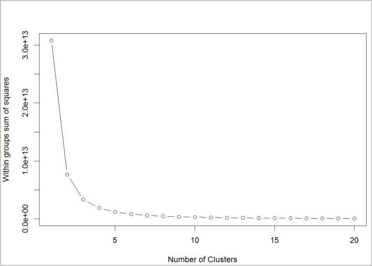
Based on the graph, it looks like k = 4 would be a good value to try. That k value will group the customers into four clusters.
Perform clustering
In the following R script, you'll use the function kmeans to perform clustering.
# Output table to hold the customer group mappings.
# Generate clusters using Kmeans and output key / cluster to a table
# called return_cluster

## create clustering model
clust <- kmeans(customer_data[,2:5],4)

## create clustering output for table
customer_cluster <- data.frame(cluster=clust$cluster,customer=customer_data$customer,orderRatio=customer_data$orderRatio,
        itemsRatio=customer_data$itemsRatio,monetaryRatio=customer_data$monetaryRatio,frequency=customer_data$frequency)

## write cluster output to DB table
sqlSave(ch, customer_cluster, tablename = "return_cluster")

# Read the customer returns cluster table from the database
customer_cluster_check <- sqlFetch(ch, "return_cluster")

head(customer_cluster_check)
Analyze the results
Now that you've done the clustering using K-Means, the next step is to analyze the result and see if you can find any actionable information.
#Look at the clustering details to analyze results
clust[-1]
$centers
   orderRatio itemsRatio monetaryRatio frequency
1 0.621835791  0.1701519    0.35510836  1.009025
2 0.074074074  0.0000000    0.05886575  2.363248
3 0.004807692  0.0000000    0.04618708  5.050481
4 0.000000000  0.0000000    0.00000000  0.000000

$totss
[1] 40191.83

$withinss
[1] 19867.791   215.714   660.784     0.000

$tot.withinss
[1] 20744.29

$betweenss
[1] 19447.54

$size
[1]  4543   702   416 31675

$iter
[1] 3

$ifault
[1] 0
The four cluster means are given using the variables defined in part two:
- orderRatio = return order ratio (total number of orders partially or fully returned versus the total number of orders)
- itemsRatio = return item ratio (total number of items returned versus the number of items purchased)
- monetaryRatio = return amount ratio (total monetary amount of items returned versus the amount purchased)
- frequency = return frequency
Data mining using K-Means often requires further analysis of the results, and further steps to better understand each cluster, but it can provide some good leads. Here are a couple ways you could interpret these results:
- Cluster 1 (the largest cluster) seems to be a group of customers that are not active (all values are zero).
- Cluster 3 seems to be a group that stands out in terms of return behavior.
Clean up resources
If you're not going to continue with this tutorial, delete the tpcxbb_1gb database.
Next steps
In part three of this tutorial series, you learned how to:
- Define the number of clusters for a K-Means algorithm
- Perform clustering
- Analyze the results
To deploy the machine learning model you've created, follow part four of this tutorial series: