Design and implement a data partitioning scheme
Data partitioning directly affects how efficiently your queries run and how much compute resources you consume. When you partition a table, you divide data into discrete segments based on column values, allowing the query engine to read only relevant portions of your dataset. This approach, called partition pruning, can dramatically reduce data scans when filters align with partition boundaries.
Consider a retail company processing millions of daily sales transactions. Analysts frequently query data by date ranges to generate weekly reports, compare month-over-month trends, and analyze seasonal patterns. Without partitioning, every query scans the entire transaction history. With proper partitioning by date, queries for a specific week touch only a fraction of the stored files.
Determine when partitioning applies
Databricks recommends that you don't partition tables containing less than 1 TB of data. For smaller tables, the overhead of managing partition metadata and the potential for creating many small files outweighs any query performance benefits. Unpartitioned Delta tables in recent Databricks Runtime versions automatically benefit from ingestion time clustering, which provides similar query advantages without explicit configuration.
When your tables exceed 1 TB, partitioning becomes a valuable optimization technique. At this scale, the benefits of reading only relevant data segments significantly offset the costs of partition management. Partitioning also enables parallel processing, as Spark can distribute different partitions across cluster nodes for concurrent execution.
Important
Each partition should contain at least 1 GB of data. This guideline helps you avoid over-partitioning, which creates excessive small files and degrades query performance.
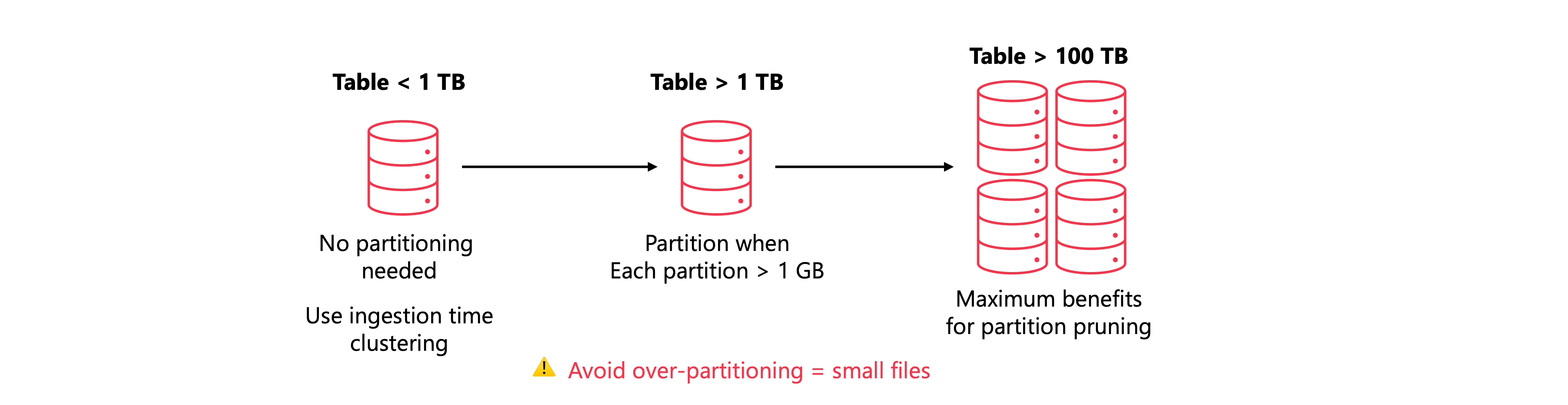
For very large tables in the hundreds of terabytes range, partitioning delivers even greater benefits. At this scale, partition pruning dramatically reduces the amount of data the query engine needs to process, improving both performance and cost efficiency.
Choose effective partition keys
Partition key selection requires you to understand your data characteristics and query patterns. Effective partition keys share common traits that maximize performance benefits while avoiding common pitfalls.
Low cardinality columns work best
Choose columns with a limited number of distinct values. Date columns, geographic regions, product categories, and status fields make excellent partition keys because they create a manageable number of partitions. A column with thousands or millions of unique values, like customer ID or transaction ID, leads to over-partitioning and poor performance.
For example, partitioning a sales table by sale_date at the daily level might create 365 partitions per year. If each day contains sufficient data volume, this granularity works well. However, partitioning by sale_timestamp at the second level would create millions of partitions, each containing minimal data.
Align with query patterns
Your partition key should match the columns that users filter on most frequently. If analysts consistently query sales data by date ranges, partitioning by date enables efficient pruning. If queries primarily filter by region, consider region as your partition key instead.
When multiple filter patterns exist, prioritize the most common or most performance-critical queries. You can define one partitioning scheme per table, so choose columns that benefit the majority of your workload. For significantly different query patterns, consider creating separate optimized materialized views or summary tables for specific use cases.
Consider data growth over time
Select a partition scheme that scales appropriately as your data grows. Partitioning by year works well initially but might create partitions that are too large over time. Conversely, partitioning by hour might work for high-volume data but creates too many small partitions for moderate volumes.
Evaluate your expected data growth rate when choosing partition granularity. A balance between partition size and the number of partitions helps maintain consistent query performance as your dataset expands.
Also consider data distribution across partitions. Severely uneven partition sizes can create processing bottlenecks, as nodes handling larger partitions take longer to complete while others remain idle.
Implement partitions in Azure Databricks
You define partitions when creating a table using the PARTITIONED BY clause in SQL or the partitionBy method in PySpark. Once you establish partitions, Azure Databricks automatically routes incoming data to the appropriate partition directories based on column values.
Create a partitioned table with SQL
The following example creates a sales transactions table partitioned by the transaction date:
CREATE TABLE sales.transactions (
    transaction_id STRING,
    customer_id STRING,
    product_id STRING,
    quantity INT,
    unit_price DECIMAL(10,2),
    total_amount DECIMAL(12,2),
    transaction_date DATE
)
PARTITIONED BY (transaction_date);
When you query this table with a date filter, the query engine reads only the partitions that match your filter criteria:
SELECT product_id, SUM(total_amount) AS revenue
FROM sales.transactions
WHERE transaction_date BETWEEN '2024-01-01' AND '2024-01-31'
GROUP BY product_id;
Create a partitioned table with PySpark
When using PySpark, specify partitioning during the write operation:
df.write.format("delta") \
    .partitionBy("transaction_date") \
    .saveAsTable("sales.transactions")
For subsequent writes, maintain consistency by including the same partition specification:
new_transactions_df.write.format("delta") \
    .mode("append") \
    .partitionBy("transaction_date") \
    .saveAsTable("sales.transactions")
Use generated columns for partition flexibility
Generated columns provide a way to derive partition values from existing columns without storing redundant data. This approach is useful when your source data contains timestamps but you want to partition by date:
CREATE TABLE sales.transactions (
    transaction_id STRING,
    customer_id STRING,
    product_id STRING,
    quantity INT,
    unit_price DECIMAL(10,2),
    total_amount DECIMAL(12,2),
    transaction_timestamp TIMESTAMP,
    transaction_date DATE GENERATED ALWAYS AS (CAST(transaction_timestamp AS DATE))
)
PARTITIONED BY (transaction_date);
Tip
With this configuration, Delta Lake automatically generates partition filters when you query using the base timestamp column. A query filtering on transaction_timestamp benefits from partition pruning without requiring explicit date filters.
Avoid common partitioning mistakes
Understanding what to avoid is as important as knowing what to do. Several common mistakes can significantly degrade performance and complicate data management.
Over-partitioning creates small file problems
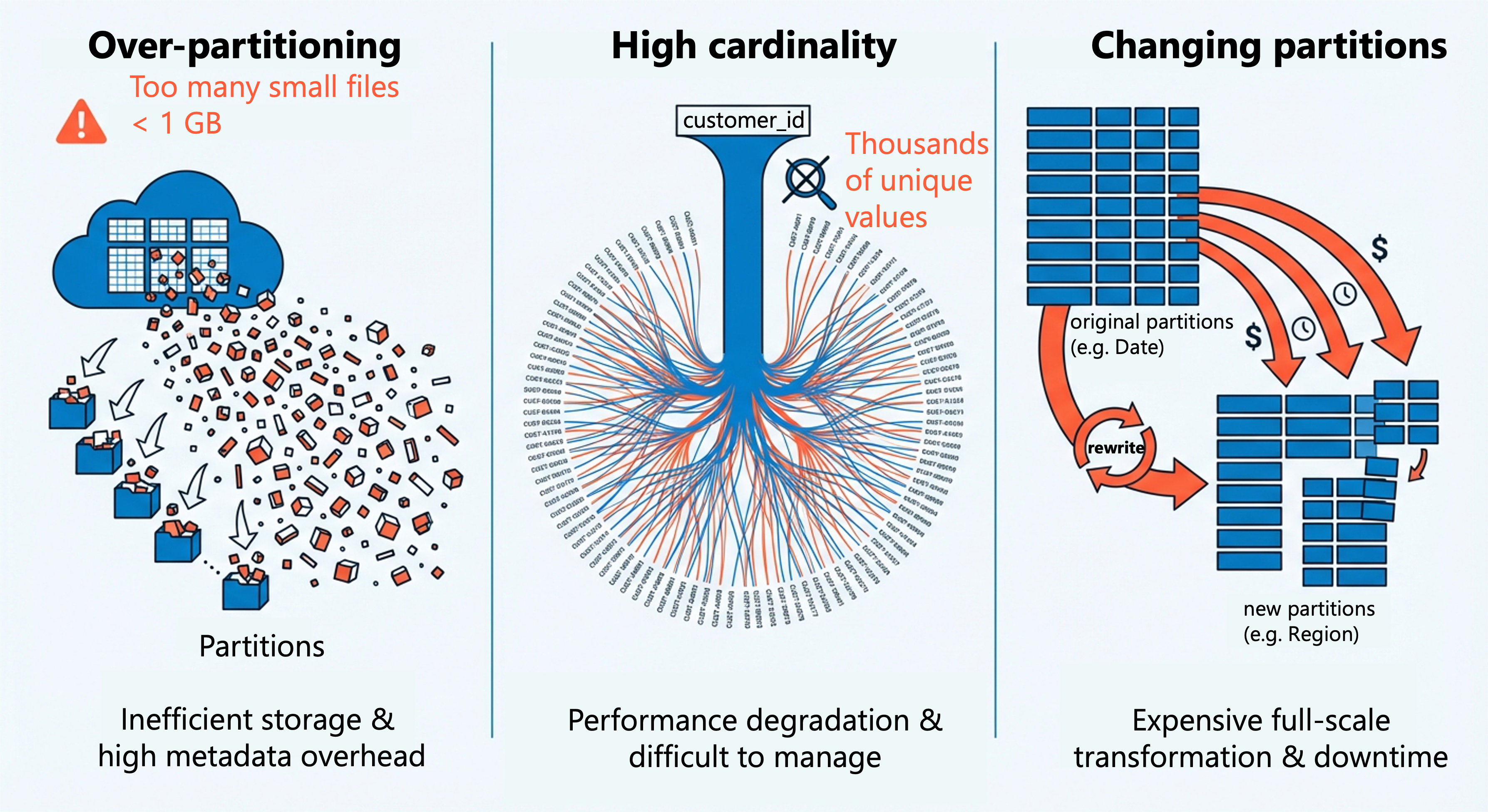
Creating too many partitions, each containing insufficient data, leads to small file problems. When partitions contain files smaller than the target file size, query performance suffers from excessive metadata operations and reduced read efficiency. Aim for partitions with at least 1 GB of data.
Signs of over-partitioning include slow query performance despite partition pruning, a large number of small files in partition directories, and long table optimization times. If you observe these symptoms, consider choosing a coarser partition granularity.
Partitioning on high-cardinality columns fails
Columns with many unique values make poor partition keys. Partitioning by customer ID, transaction ID, or other high-cardinality columns creates millions of partitions that degrade rather than improve performance. Reserve high-cardinality column optimization for other techniques that are designed for this purpose.
Changing partitions requires rewriting data
Partition columns are part of the table structure. Changing your partitioning strategy requires rewriting the entire table to a new location with different partition boundaries. This operation consumes significant compute resources and time for large tables.
Plan your partitioning strategy carefully before loading data at scale. Consider future query patterns and data growth to avoid costly restructuring later.
Document partitioning decisions
Record your partition key choices and the reasoning behind them. This documentation helps team members understand query optimization opportunities and prevents accidental changes that could impact performance. Include information about expected partition sizes, query patterns that benefit from the scheme, and any constraints that influenced your decisions.
Consider liquid clustering as an alternative
When you encounter partitioning challenges—especially with high-cardinality columns like timestamps or when query patterns are uncertain—liquid clustering provides a modern alternative. Unlike traditional partitioning, liquid clustering offers:
- Flexibility to adjust optimization strategies without rewriting data
- Automatic maintenance as tables grow
- Reduced partition management overhead
Liquid clustering is the recommended approach for new tables where partitioning constraints would limit performance or create excessive maintenance burden. It's particularly effective for tables that exceed 1 TB and require filtering on columns that would create too many partitions using traditional approaches.
Note
Liquid clustering is not compatible with partitioned tables. Choose one approach based on your requirements when designing new tables.
For implementation details, syntax, and optimization strategies, refer to the Design and implement a clustering strategy unit later in this module.