Introduction to image data
- 10 minutes
In computer vision, we normally solve one of the following problems:
- Image Classification is the simplest task, when we need to classify an image into one of many predefined categories, for example, distinguish a cat from a dog on a photograph, or recognize a handwritten digit.
- Object Detection is a bit more difficult task, in which we need to find known objects on the picture and localize them, that is, return the bounding box for each of recognized objects.
- Segmentation is similar to object detection, but instead of giving bounding box we need to return an exact pixel map outlining each of the recognized objects.
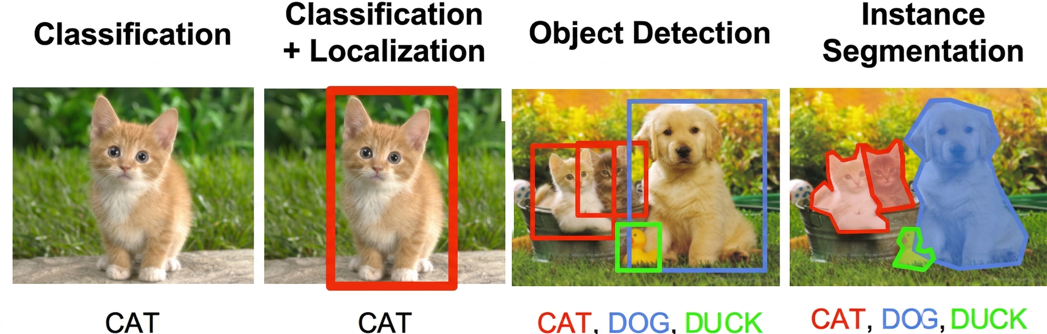
Image from CS231n Stanford Course
Images as tensors
Computer Vision works with Images. As you probably know, images consist of pixels, so they can be thought of as a rectangular collection (array) of pixels.
In the first part of this module, we'll deal with handwritten digit recognition. We'll use the MNIST dataset, which consists of grayscale images of handwritten digits, 28x28 pixels. Each image can be represented as 28x28 array, and elements of this array would denote intensity of corresponding pixel - either in the scale of range 0 to 1 (in which case floating point numbers are used), or 0 to 255 (integers). A popular Python library called numpy is often used with computer vision tasks, because it allows you to operate with multidimensional arrays effectively.
To deal with color images, we need some way to represent colors. In most cases, we represent each pixel by 3 intensity values, corresponding to Red (R), Green (G), and Blue (B) components. This color encoding is called RGB, and thus color image of size W×H will be represented as an array of size H×W×3 (sometimes the order of components might be different, but the idea is the same). In array representation, the height (number of rows) comes before the width (number of columns), which is the opposite of the common image convention of W×H.
Multi-dimensional arrays are also called tensors. Using tensors to represent images also has an advantage, because we can use an extra dimension to store a sequence of images. For example, to represent a video fragment consisting of 200 frames with 800x600 dimension (width × height), we may use the tensor of size 200x600x800x3. Remember that tensor dimensions use H×W (row-major) order, not the W×H convention commonly seen in image editors. The order here's frames × height (600) × width (800) × channels. This ordering is known as channels_last and is the default in TensorFlow; some other frameworks place channels before height and width (channels_first).
import tensorflow as tf
import keras
import matplotlib.pyplot as plt
import numpy as np

# Prints the installed TensorFlow version
print(tf.__version__)
We're going to use the Keras framework for our experiments. Throughout this module, we use import keras (the standalone Keras 3 import style), which requires TensorFlow 2.16 or later (or a standalone installation via pip install keras>=3.0). If you're using an older TensorFlow 2.x version, replace import keras with from tensorflow import keras.
(x_train, y_train), (x_test, y_test) = keras.datasets.mnist.load_data()

# Output: (60000, 28, 28) (60000,)
print(x_train.shape, y_train.shape)
# Output: (10000, 28, 28) (10000,)
print(x_test.shape, y_test.shape)
Visualize the digits dataset
Now that we have downloaded the dataset we can visualize some of the digits:
fig, ax = plt.subplots(1, 7)
for i in range(7):
    ax[i].imshow(x_train[i])
    ax[i].set_title(y_train[i])
    ax[i].axis('off')
# Displays a row of seven handwritten digit images with their labels
Dataset structure
We have a total of 60,000 training images and 10,000 test images, and each image has a size of 28×28 pixels:
print('Training samples:', len(x_train))
print('Test samples:', len(x_test))
print('Tensor size:', x_train[0].shape)
print('First 10 digits are:', y_train[:10])
print('Type of data is ', type(x_train))
# Output:
# Training samples: 60000
# Test samples: 10000
# Tensor size: (28, 28)
# First 10 digits are: [5 0 4 1 9 2 1 3 1 4]
# Type of data is  <class 'numpy.ndarray'>
As you can see, the type of data is numpy array. Each pixel intensity is represented by an integer value between 0 and 255:
print('Min intensity value: ', x_train.min())
print('Max intensity value: ', x_train.max())
# Output:
# Min intensity value:  0
# Max intensity value:  255
The reason it is between 0 and 255 is because each pixel is represented by an 8-bit integer. In many cases, especially when working with neural networks, it's more convenient to scale all values to the range [0, 1] by dividing by 255. This process is called normalization:
x_train = x_train.astype(np.float32) / 255.0
x_test = x_test.astype(np.float32) / 255.0
# Pixel values are now floating point numbers in the range [0, 1]
Now we have the data, and we're ready to start training our first neural network!
Check your knowledge
Feedback
Was this page helpful?
No
Need help with this topic?
Want to try using Ask Learn to clarify or guide you through this topic?