Previous

Next

Convolutional neural networks

Completed

While you can use deep learning models for any kind of machine learning, they're particularly useful for dealing with data that consists of large arrays of numeric values - such as images. Machine learning models that work with images are the foundation for an area artificial intelligence called computer vision, and deep learning techniques have been responsible for driving amazing advances in this area over recent years.

At the heart of deep learning's success in this area is a kind of model called a convolutional neural network, or CNN. A CNN typically works by extracting features from images, and then feeding those features into a fully connected neural network to generate a prediction. The feature extraction layers in the network have the effect of reducing the number of features from the potentially huge array of individual pixel values to a smaller feature set that supports label prediction.

Layers in a CNN

CNNs consist of multiple layers, each performing a specific task in extracting features or predicting labels.

Convolution layers

One of the principal layer types is a convolutional layer that extracts important features in images. A convolutional layer works by applying a filter to images. The filter is defined by a kernel that consists of a matrix of weight values.

For example, a 3x3 filter might be defined like this:

 1  -1   1
-1   0  -1
 1  -1   1

An image is also just a matrix of pixel values. To apply the filter, you "overlay" it on an image and calculate a weighted sum of the corresponding image pixel values under the filter kernel. The result is then assigned to the center cell of an equivalent 3x3 patch in a new matrix of values that is the same size as the image. For example, suppose a 6 x 6 image has the following pixel values:

255 255 255 255 255 255 
255 255 100 255 255 255
255 100 100 100 255 255
100 100 100 100 100 255
255 255 255 255 255 255
255 255 255 255 255 255

Applying the filter to the top-left 3x3 patch of the image would work like this:

255 255 255      1  -1   1    (255 x 1)+(255 x -1)+(255 x 1) +
255 255 100  x  -1   0  -1  = (255 x -1)+(255 x 0)+(100 x -1) +   = 155
255 100 100      1  -1   1    (255 x1 )+(100 x -1)+(100 x 1)

The result is assigned to the corresponding pixel value in the new matrix like this:

 ?   ?   ?   ?   ?   ?  
 ?  155  ?   ?   ?   ?
 ?   ?   ?   ?   ?   ?
 ?   ?   ?   ?   ?   ?
 ?   ?   ?   ?   ?   ?
 ?   ?   ?   ?   ?   ?

Now the filter is moved along (convolved), typically using a step size of 1 (so moving along one pixel to the right), and the value for the next pixel is calculated

255 255 255      1  -1   1    (255 x 1)+(255 x -1)+(255 x 1) +
255 100 255  x  -1   0  -1  = (255 x -1)+(100 x 0)+(255 x -1) +   = -155
100 100 100      1  -1   1    (100 x1 )+(100 x -1)+(100 x 1)

So now we can fill in the next value of the new matrix.

 ?   ?   ?   ?   ?   ?  
 ?  155 -155 ?   ?   ?
 ?   ?   ?   ?   ?   ?
 ?   ?   ?   ?   ?   ?
 ?   ?   ?   ?   ?   ?
 ?   ?   ?   ?   ?   ?

The process repeats until we've applied the filter across all of the 3x3 patches of the image to produce a new matrix of values like this:

?   ?   ?    ?    ?   ?
?  155 -155 155 -155  ?
? -155 310 -155  155  ?
?  310 155  310   0   ?
? -155 -155 -155  0   ?
?   ?   ?    ?    ?   ?

Because of the size of the filter kernel, we can't calculate values for the pixels at the edge; so we typically just apply a padding value (often 0):

0   0   0    0    0   0
0  155 -155 155 -155  0
0 -155 310 -155  155  0
0  310 155  310   0   0
0 -155 -155 -155  0   0
0   0   0    0    0   0

The output of the convolution is typically passed to an activation function, which is often a Rectified Linear Unit (ReLU) function that ensures negative values are set to 0:

0   0   0    0    0   0
0  155  0   155   0   0
0   0  310   0   155  0
0  310 155  310   0   0
0   0   0    0    0   0
0   0   0    0    0   0

The resulting matrix is a feature map of feature values that can be used to train a machine learning model.

Note: The values in the feature map can be greater than the maximum value for a pixel (255), so if you wanted to visualize the feature map as an image you would need to normalize the feature values between 0 and 255.

The convolution process is shown in the animation below.

1. An image is passed to the convolutional layer. In this case, the image is a simple geometric shape.
2. The image is composed of an array of pixels with values between 0 and 255 (for color images, this is usually a 3-dimensional array with values for red, green, and blue channels).
3. A filter kernel is generally initialized with random weights (in this example, we've chosen values to highlight the effect that a filter might have on pixel values; but in a real CNN, the initial weights would typically be generated from a random Gaussian distribution). This filter will be used to extract a feature map from the image data.
4. The filter is convolved across the image, calculating feature values by applying a sum of the weights multiplied by their corresponding pixel values in each position. A Rectified Linear Unit (ReLU) activation function is applied to ensure negative values are set to 0.
5. After convolution, the feature map contains the extracted feature values, which often emphasize key visual attributes of the image. In this case, the feature map highlights the edges and corners of the triangle in the image.

Typically, a convolutional layer applies multiple filter kernels. Each filter produces a different feature map, and all of the feature maps are passed onto the next layer of the network.

Pooling layers

After extracting feature values from images, pooling (or downsampling) layers are used to reduce the number of feature values while retaining the key differentiating features that have been extracted.

One of the most common kinds of pooling is max pooling in which a filter is applied to the image, and only the maximum pixel value within the filter area is retained. So for example, applying a 2x2 pooling kernel to the following patch of an image would produce the result 155.

0   0
0  155

Note that the effect of the 2x2 pooling filter is to reduce the number of values from 4 to 1.

As with convolutional layers, pooling layers work by applying the filter across the whole feature map. The animation below shows an example of max pooling for an image map.

1. The feature map extracted by a filter in a convolutional layer contains an array of feature values.
2. A pooling kernel is used to reduce the number of feature values. In this case, the kernel size is 2x2, so it will produce an array with quarter the number of feature values.
3. The pooling kernel is convolved across the feature map, retaining only the highest pixel value in each position.

Dropping layers

One of the most difficult challenges in a CNN is the avoidance of overfitting, where the resulting model performs well with the training data but doesn't generalize well to new data on which it wasn't trained. One technique you can use to mitigate overfitting is to include layers in which the training process randomly eliminates (or "drops") feature maps. This may seem counterintuitive, but it's an effective way to ensure that the model doesn't learn to be over-dependent on the training images.

Other techniques you can use to mitigate overfitting include randomly flipping, mirroring, or skewing the training images to generate data that varies between training epochs.

Flattening layers

After using convolutional and pooling layers to extract the salient features in the images, the resulting feature maps are multidimensional arrays of pixel values. A flattening layer is used to flatten the feature maps into a vector of values that can be used as input to a fully connected layer.

Fully connected layers

Usually, a CNN ends with a fully connected network in which the feature values are passed into an input layer, through one or more hidden layers, and generate predicted values in an output layer.

A basic CNN architecture might look similar to this:

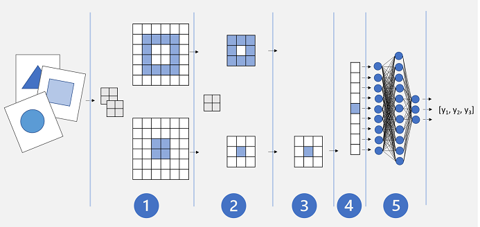
1. Images are fed into a convolutional layer. In this case, there are two filters, so each image produces two feature maps.
2. The feature maps are passed to a pooling layer, where a 2x2 pooling kernel reduces the size of the feature maps.
3. A dropping layer randomly drops some of the feature maps to help prevent overfitting.
4. A flattening layer takes the remaining feature map arrays and flattens them into a vector.
5. The vector elements are fed into a fully connected network, which generates the predictions. In this case, the network is a classification model that predicts probabilities for three possible image classes (triangle, square, and circle).

Training a CNN model

As with any deep neural network, a CNN is trained by passing batches of training data through it over multiple epochs, adjusting the weights and bias values based on the loss calculated for each epoch. In the case of a CNN, backpropagation of adjusted weights includes filter kernel weights used in convolutional layers as well as the weights used in fully connected layers.

Continue