"External Data Refresh Failed" when refreshing Project Online data in Excel Online

This article was written by Tom Schauer, Technical Specialist.

Symptoms

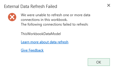
When you try to refresh Project Online data in Excel Online, the refresh fails. Additionally, you receive the following error message:

External Data Refresh Failed.

Cause

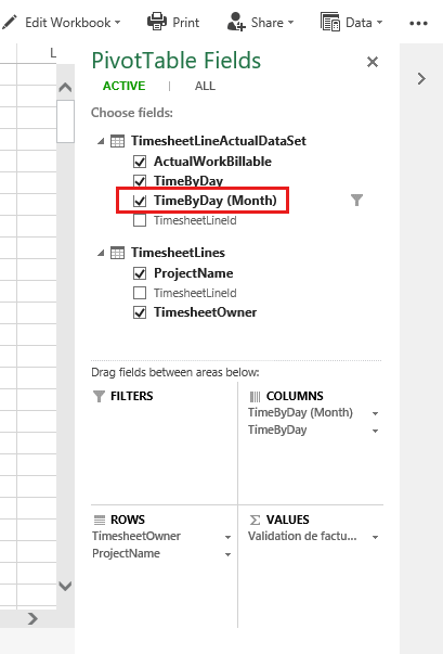
This issue occurs if you select the TimeByDay (Month) option in PivotTable Fields.

Resolution

If you clear the TimeByDay (Month) option, the error will not occur when you refresh Excel Online. However, your workbook may not look the way that you want it to look. To fix this, follows these steps:

1. In Excel, select File > Options > Data.

2. Select the Disable automatic grouping of Date/Time columns in PivotTables check box, and then select OK.

   

3. Remove the existing "TimeByDay" columns in Power Pivot. To do this, select the Power Pivot tab, and then select Manage. In the Power Pivot for Excel window, you see two columns on the Home tab that are named TimeByDay (Month Index) and TimeByDay (Month). Select both columns, right-click both columns, and then select Delete Columns.

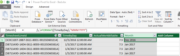
4. After you remove the auto-generated time columns, select Add Column, name it as Month, and then add the following formula to this column:

   =FORMAT([TimeByDay],"MMM YYYY")

   

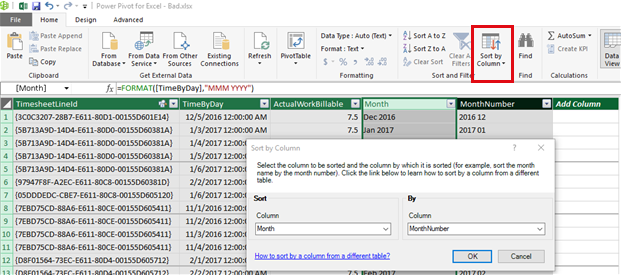
5. Select Add Column again, name it as MonthNumber, and then add the following formula to this column:

   =FORMAT([TimeByDay],"YYYY MM")

   

6. Sort the Month column by MonthNumber. To do this, select the Month column, select Sort by Column, and then select MonthNumber in the Sort by Column window.

   

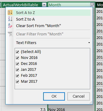
7. On the Month column, select Sort A to Z. This sorts the months in the correct chronological and alphabetical order.

   

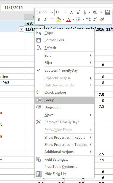
8. Go back to your Pivot table, select one cell of the TimeByDay column, and then select Group.

   

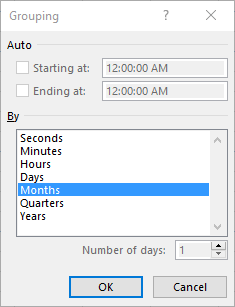
9. Select Months > OK.

   

You now have the appearance of using the TimeByDay (Month) field.